Note: GIFs will not load in .pdf version.
Before creating a neural radiance field, we first explore a simpler way of reconstructing images using a neural network. In this section, we implement a simple MLP with positional encoding to predict pixel values of a 2D image.
The MLP is structured as outlined in the spec, using a positional encoding layer, three linear layers with ReLU activations, and a final linear layer with a sigmoid activation to constrain the outputs to be between 0 and 1 - RGB values.

The positional encoding layer is constructed to expand out the dimensionality of our input coordinates. Alongside the original coordinates, we add different low and high frequency components, created using the following equation: $$ PE(x) = \{x, \sin(2^0 \pi x), \cos(2^0 \pi x), \sin(2^1 \pi x), \cos(2^1 \pi x), \cdots, \sin(2^{L-1} \pi x), \cos(2^{L-1} \pi x)\} $$ Applied to both the $x$ and $y$ coordinate. The dimensionality of the output depends on the highest frequency level $L$. For this part, we choose $L = 10$. So we take a 2D input, and generate a 42 dimension vector (2 for original dimensions, 20 for $x$ components, 20 for $y$ components).
To train the network, we sample $N$ pixels (in this stage $N = 10000$) without replacement, and propogate them through the network. Coordinates are normalized to between 0 and 1, and to calculate the loss, the corresponding RGB vectors are also normalized so each component is in $[0, 1]$.
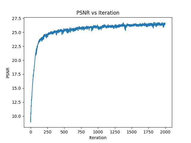
To train, we use MSE loss, but use PSNR (peak signal-to-noise ratio) to manually assess the quality of our reconstructed image, where: $$PSNR = 10 \cdot \log_{10} \left ( \frac{1}{MSE} \right )$$ Following the spec, I started with Adam as the optimizer, with a learning rate of 1e-2, a batch size of 10000 as mentioned above, a hidden layer size of 256, over 2000 iterations. Below are the results:
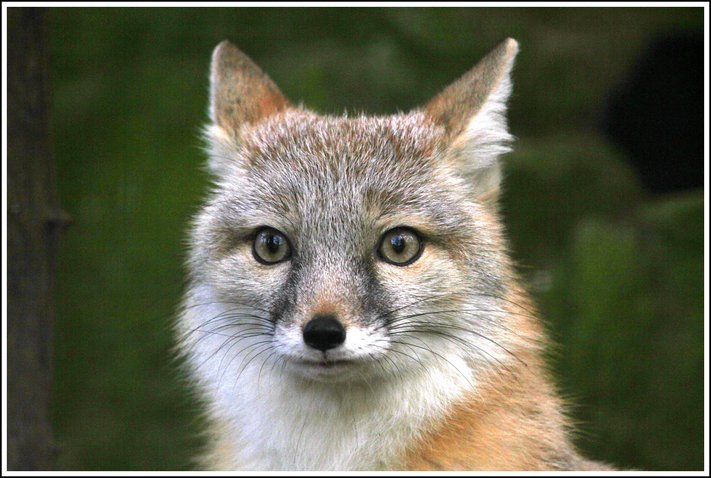
We begin by training the neural net to reconstruct this following image:
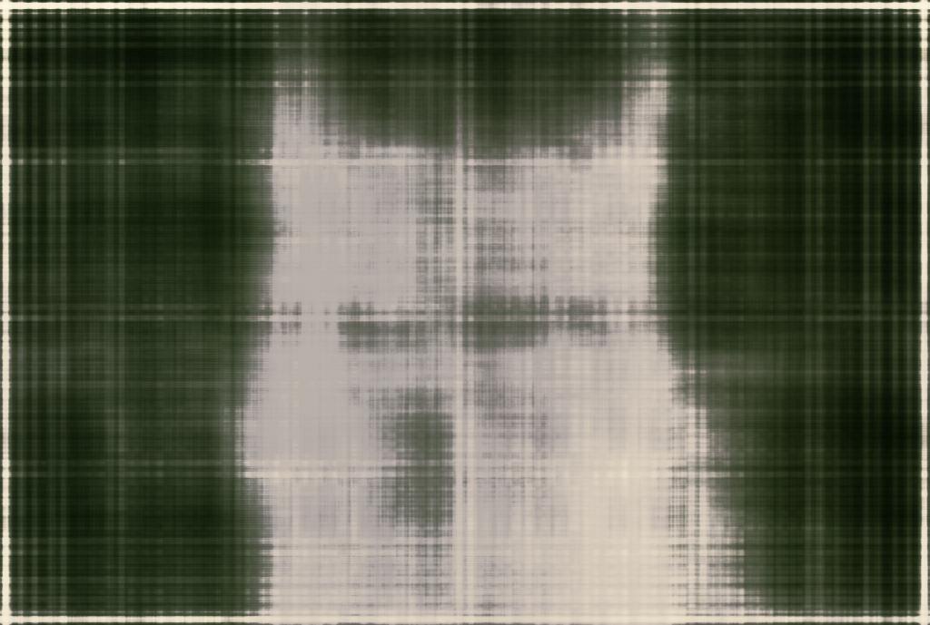
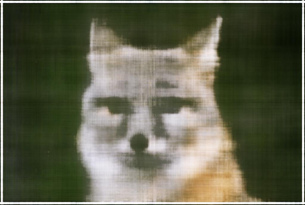
Tracking the progress after several iterations, this is what we get:

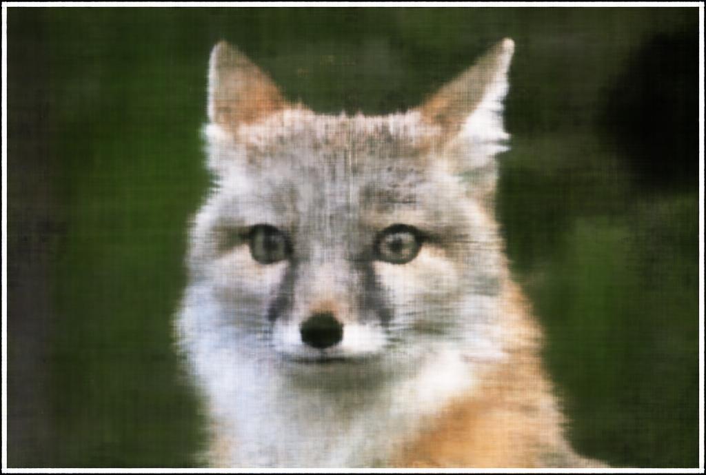
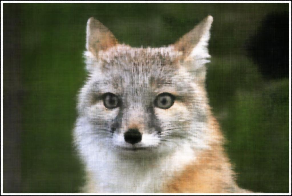
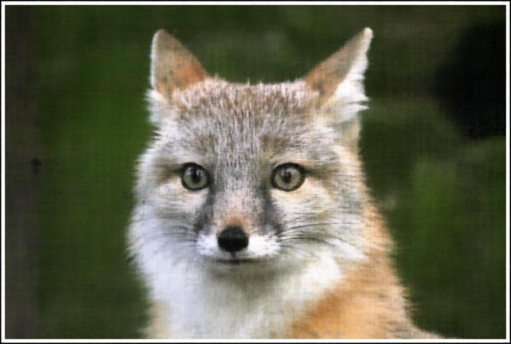
We can also observe the training PSNR curve over all 2000 iterations:
Next, I tried some different hyperparameters. I specifically altered the max frequency of the positional encoding by doubling it to $L = 20$, and subsequently also lowered the learning rate. The idea was that higher frequency levels could add addition information about high frequency/more detailed features in the original image, and a lower learning rate would help avoid the plateau in PSNR later in the training process.
This resulted in the following images and 1000 and 2000 iterations, side by side with their default counterparts:
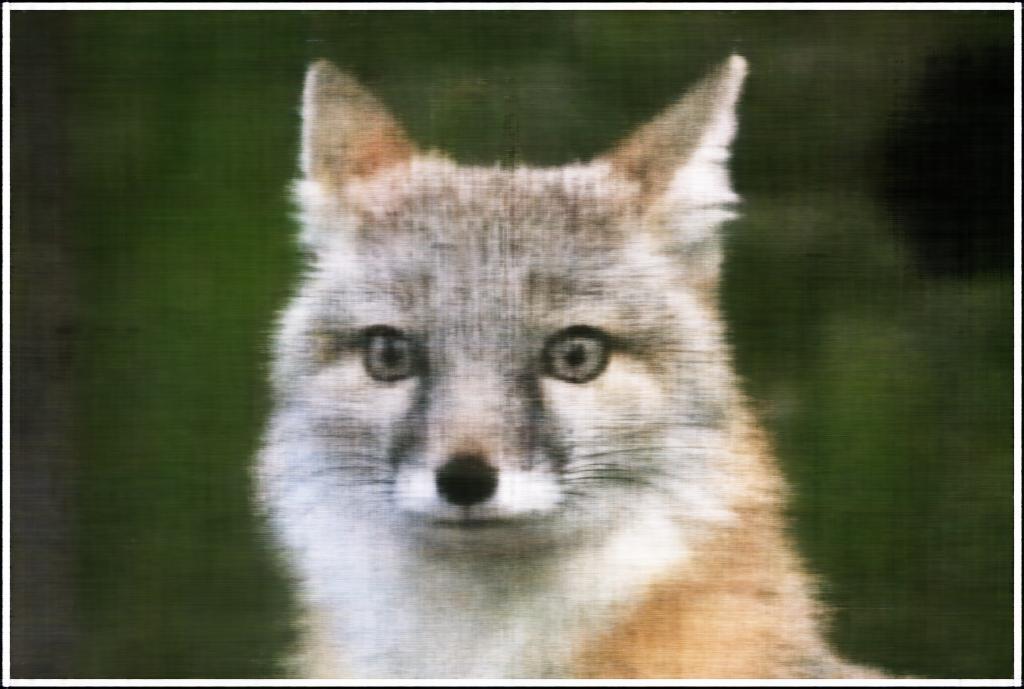

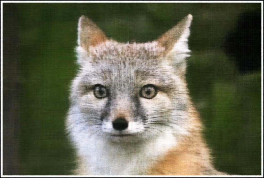

Overall, the defaults seemed better, capturing more of the details on the fur. We can also compare the two PSNR curves, shown below:
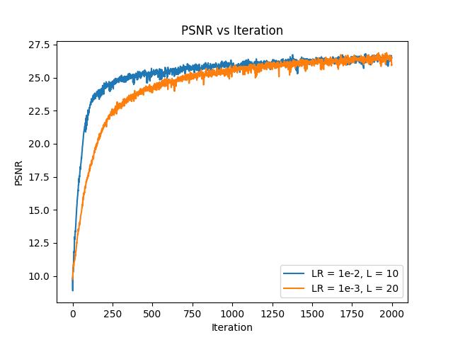
The lower learning rate leads the alternative hyperparameters (in orange) to coverge more slowly but they end up at around the same place after 2000 iterations.
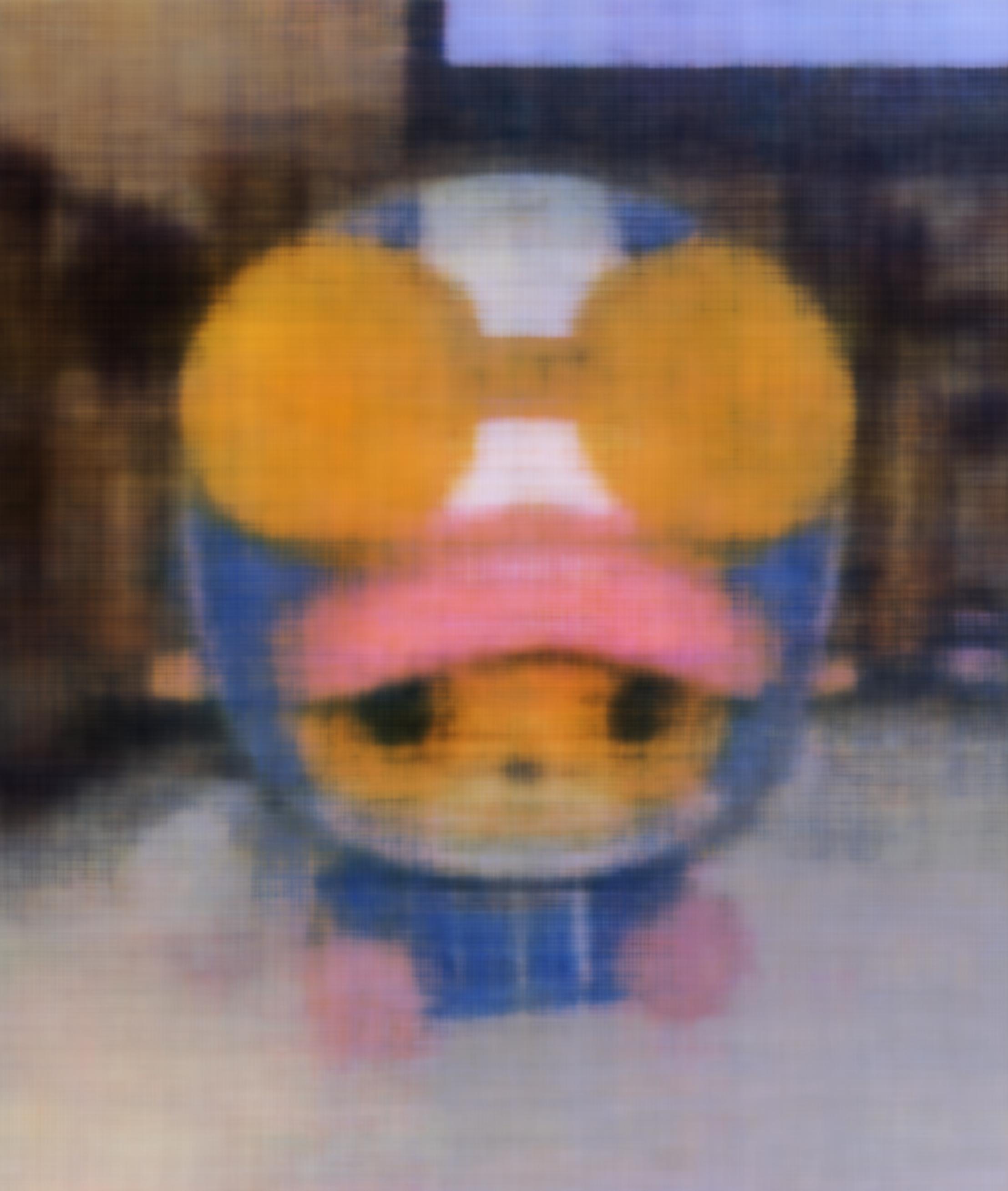
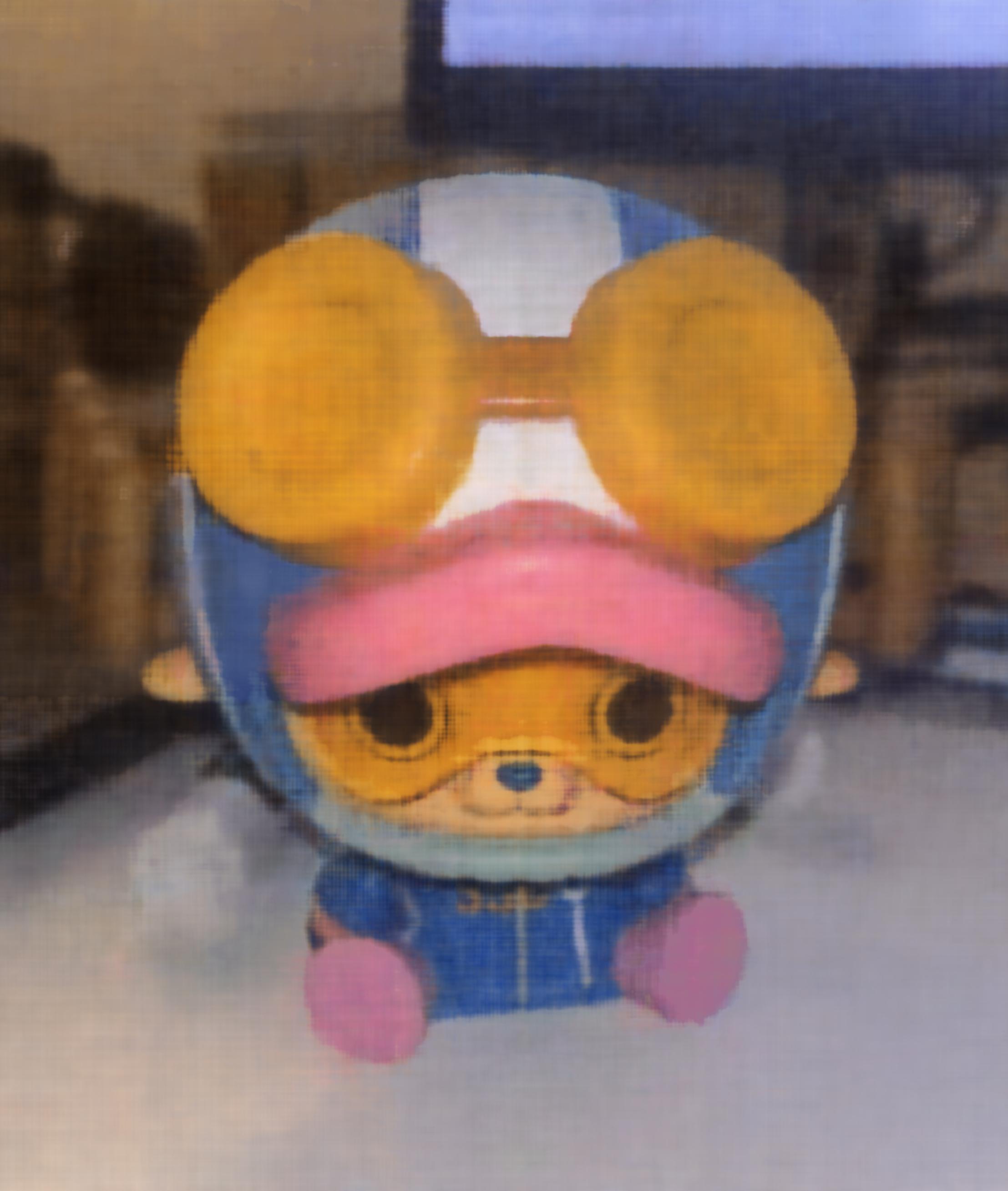
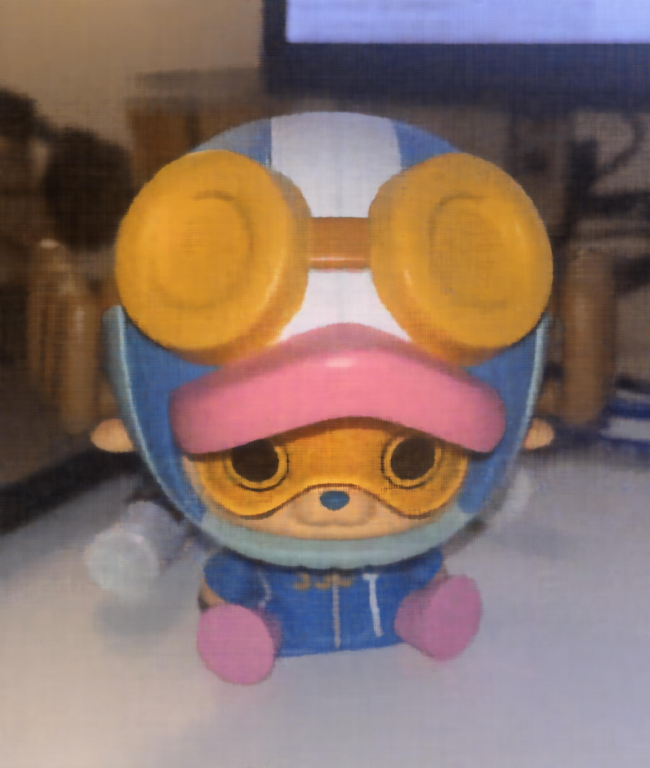
Next, we test the MLP on a custom picture - I chose an image of a figurine on my desk, which was higher definition than the test image.
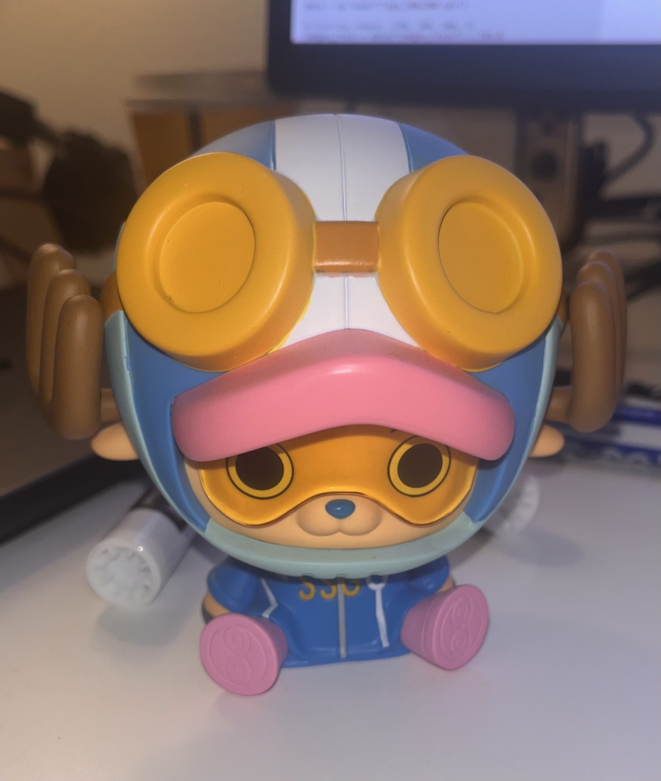
Below are the results for training using the default hyperparameters (LR = 1e-2, $L = 10$, hidden layer size = 256), but instead only up to 1000 iterations:

Below is the training PSNR curve for the new custom image:
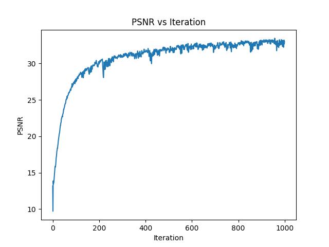
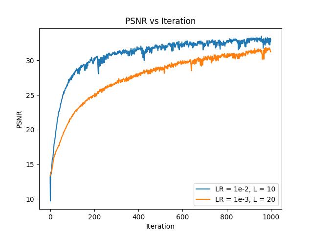
Again, we can try the alternative hyperparameters (LR = 1e-3, $L = 20$) to see if they can improve performance, particularly on a larger image:


The default hyperparameters are pretty evidently better, which is supported by the compared PSNR curve:
Having done some testing on a simplified MLP used for predicting 2D coordinate RGB values, we can now expand it to predict 3D world coordinate RGB values + density.
For this portion of the project, we are given a set of images of the same object (a lego set) from various viewpoints, along with each images' corresponding camera-to-world transformation matrix, and a set focal length. To begin constructing a neural radiance field, we first need to write some helper functions that can help us translate from pixel coordinates to rays.
First, we need to create a function that can transform coordinates in camera space to coordinates in world space. Since we're given the c2w matrices, this is relatively simple: $$ \begin{bmatrix} x_w \\ y_w \\ z_w \\ 1 \end{bmatrix} = \begin{bmatrix} \mathbf{R}_{3 \times 3} & \mathbf{t} \\ \mathbf{0}_{1 \times 3} & 1 \end{bmatrix}^{-1} \begin{bmatrix} x_c \\ y_c \\ z_c \\ 1 \end{bmatrix} $$ Where $\begin{bmatrix} \mathbf{R}_{3 \times 3} & \mathbf{t} \\ \mathbf{0}_{1 \times 3} & 1 \end{bmatrix}^{-1}$ is the c2w matrix, or the inverse of the extrinsic matric composed of rotation matrix $\mathbf{R}$ and translation vector $\mathbf{t}$.
We also want a function that can map pixel coordinates to camera coordinates. To do so, we use the intrinsic matrix of the camera $\mathbf{K}$, defined as: $$ \mathbf{K} = \begin{bmatrix} f_x & 0 & o_x \\ 0 & f_y & o_y \\ 0 & 0 & 1 \\ \end{bmatrix}^{-1} $$ Where $f_x, f_y$ are the local length, and $o_x, o_y$ are the coordinates of the center of the image, or the principal point assuming a pinhole camera.
With $\mathbf{K}$, we can now convert from pixel coordinates $(u, v)$ to 3D camera coordinates $(x_c, y_c, z_c)$ using the following equation: $$ \begin{bmatrix} x_c \\ y_c \\ z_c \\ \end{bmatrix} = s \times \mathbf{K}^{-1} \begin{bmatrix} u \\ v \\ 1 \\ \end{bmatrix} $$ Where $s$ is the depth of the 3D point along the ray (since for any one 2D pixel there are infinitely many 3D points that could correspond, along the optical axis).
Putting the previous two functions together, we can create a function that maps from pixels to rays. The origin of the ray can just be set to the location of the camera, which we can find using this equation: $$ \mathbf{r}_o = - \mathbf{R}_{3 \times 3}^{-1} \mathbf{t} $$
The directin of the ray can be represented by any point along the ray, which we can find by mapping our pixel coordinate to our camera coordinate (using the second function we defined), and then map the camera coordinate to a world coordinate which lays along the ray (using the first function we defined). In this case, the depth is arbitrary, so we can just set $s = 1$.
To ensure consitency, we finally normalize the ray direction (since any point along the ray can define a valid ray direction but result in different scales), using the following equation: $$\mathbf{r}_d = \frac{\mathbf{X}_w - \mathbf{r}_o}{||\mathbf{R}_w - \mathbf{r}_o||_2}$$ Where $\mathbf{X}_w = (x_w, y_w, z_w)$.
Now, we have a function that maps from any pixel coordinate from a given camera (and its c2w matrix + focal length) to its corresponding ray in world space.
Similar to the first part, we want to train our MLP on sampled points, this time in 3D world space. The process for sampling for this section is a bit more involved, since we are now working in 3D and along rays.
First, we need to sample rays from images. To do this, we essentially sample pixels from our available images, then convert them into rays using our previously defined helper. Since we have multiple images, in my implementation I flatten all the images, randomly select pixels, retrieve their original coordinates, and use those coordinates + the corresponding c2w matrices and focal length to compute the rays.
For our MLP, we don't trai/predict on rays, but on 3D points, so our next step is to sample from the rays at consistent intervals. To do so, we essentially create linear intervals between different depth values along the ray. Following the spec, these values were selected between 2 and 6, and I chose to take 64 evenly spaced samples.
To convert from sampled depths + a ray to 3D coordinates. We can use the following formula: $\mathbf{x} = \mathbf{R}_o + \mathbf{R}_d \times t$. So each ray will produce 64 discrete samples of 3D $(x, y, z)$ coordinates in world space.
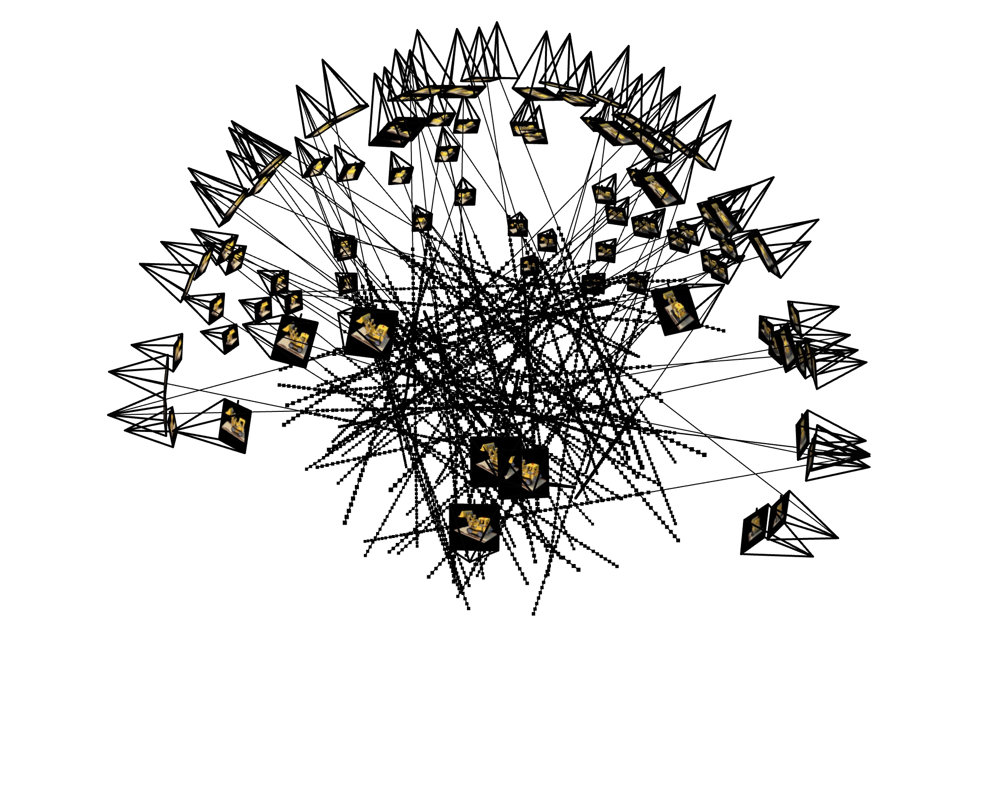
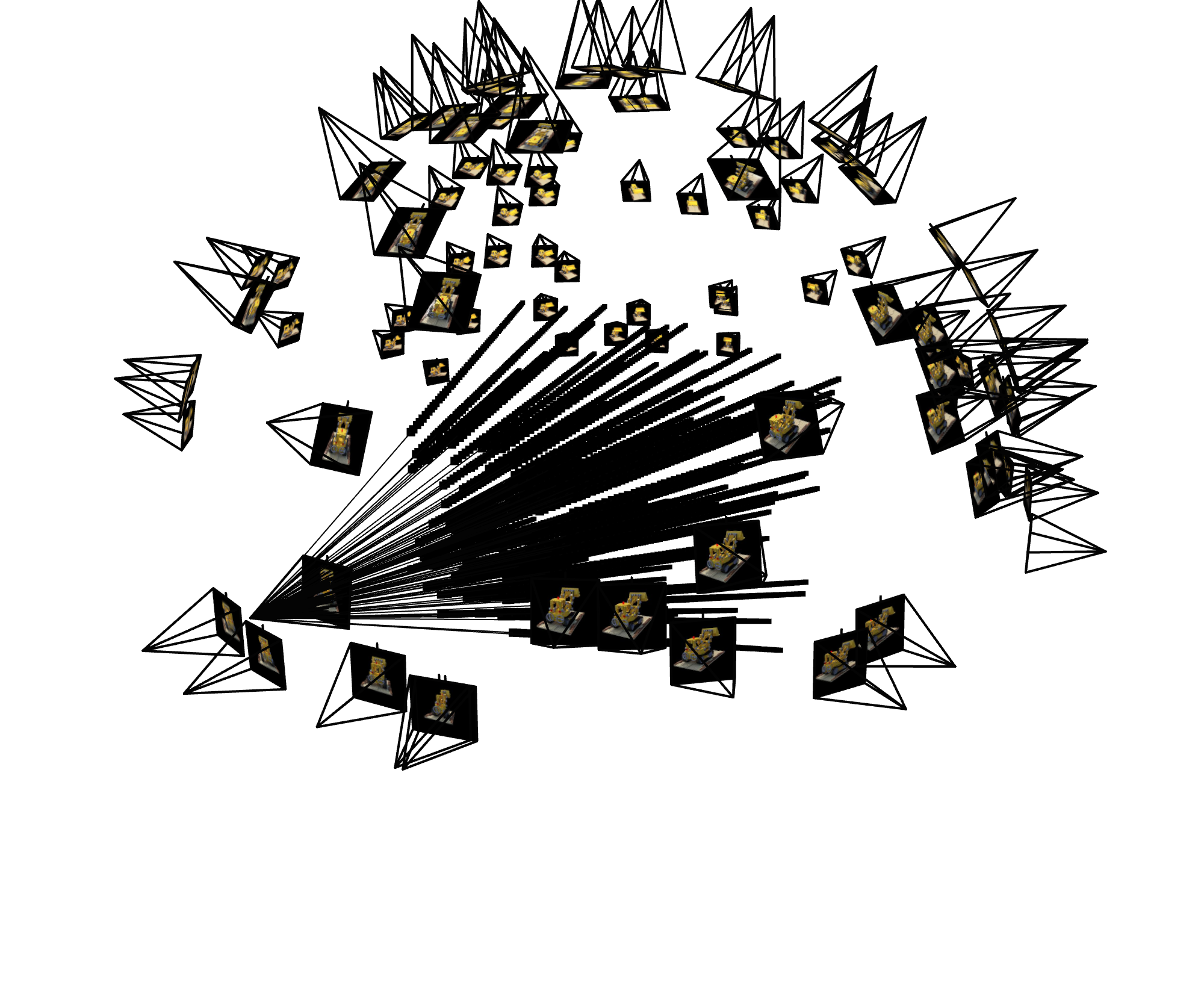
We can now visualize some of the rays generated using our sampling process using viser. Each line represents a ray, and the dots along the line represent the discrete points we sample.
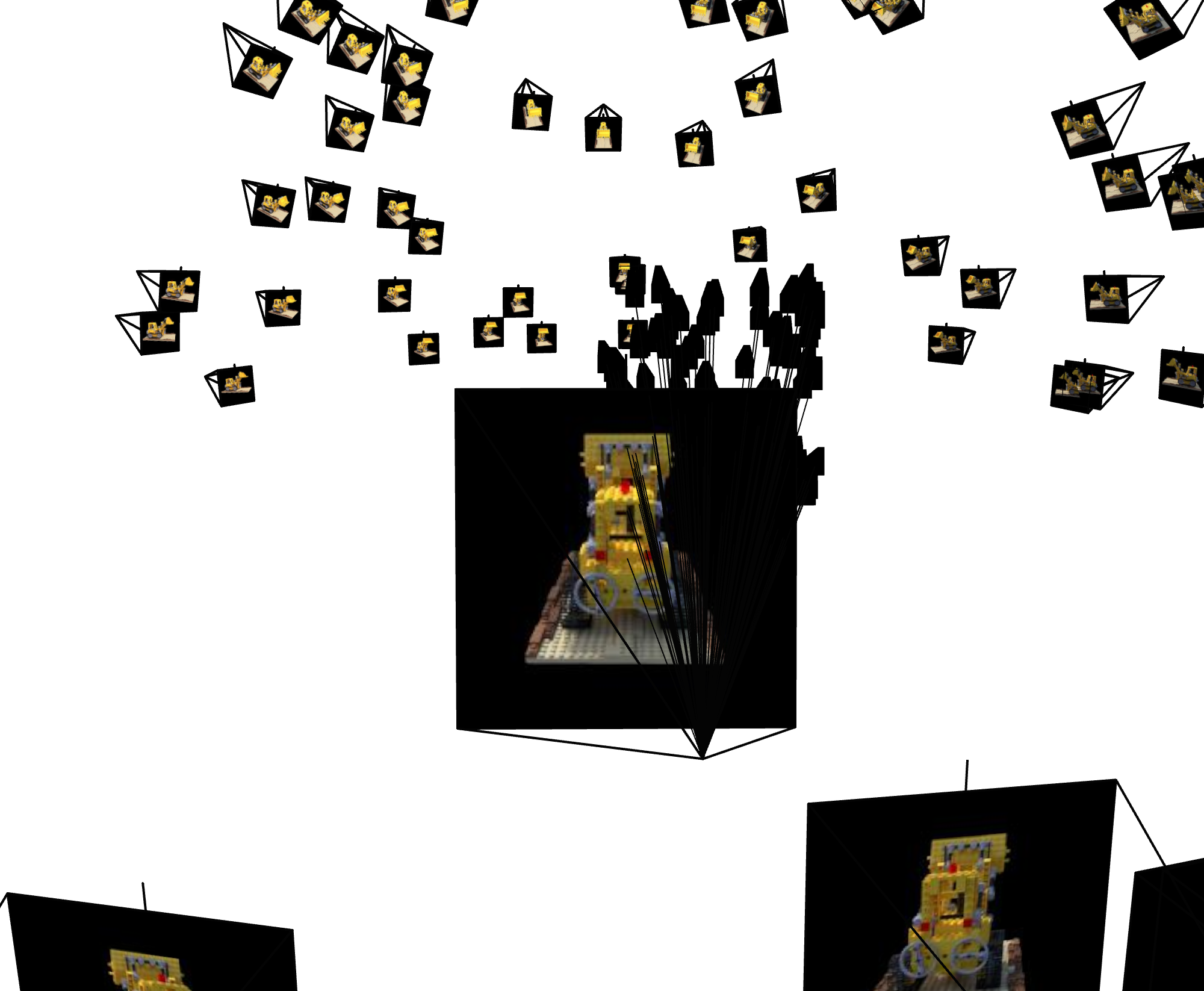
Having implemented our 3D point sampling, we can now build the general architecture of the MLP that will predict RGB values and densities. The archiecture is taken from the spec, shown below:

The positional encoding layers are the same as in part 1, except now the input is 3D, and ray direction positional encoding layer only uses $L = 4$, while the coordinate PE layer still uses $L = 10$. This means the coordinate PE layer takes in a vector of dimension 3, and outputs a vector of dimension 63 (3 + 20 * 3), and the directional PE layer takes in a vector of dimension 3, and outputs a vector of dimension 27 (3 + 8 * 3).
Since the network gets deeper, we also add some skip layers, specifically where the positionally encoded vectors are directly concatenated with later layer outputs to help the network "remember" its inputs.
The final major change other than depth is that the network now has two outputs, but the RGB value of the point, and also the density of the point, which controls how much light passes through that point/is obscured.
For both training and inference, we need a way to convert each ray (represented by its sampled points) into a single vector representing the predicted RGB value at the pixel + camera we are predicting. To do so, we use a volume rendering equation: $$C(\mathbf{r}) = \int_{t_n}^{t_f} T(t) \sigma(\mathbf{r}(t))\mathbf{c}(\mathbf{r}(t), \mathbf{d}) dt$$ Where $T(t) = \exp\left(- \int_{t_n}^t \sigma(\mathbf{r}(s)) ds\right)$
This equation essentially measures how the color from a certain point in 3D space will be reflected in our camera. This equation is discretized for computation along discrete samples aong the ray instead of infinitely small intervals: $$\hat C(\mathbf{r}) = \sum_{i = 1}^N T_i (1 - \exp(-\sigma_i \delta_i)) \mathbf{c}_i$$ Where $T(t) = \exp\left(- \sum_{j = 1}^{i - 1} \sigma(j)\delta_j \right)$.
Following the discrete equation, we can get estimations for the final color at a specific point on our imaging plane (ie our pixel value) by using the predicted RGB values and densities of the samples along the ray we derived from the pixel value. In other words, we start with a pixel -> ray -> samples along ray -> pass through MLP to get RGBs, densities -> plug all samples into volume rendering equation -> get predicted pixel value. To train the MLP, we can conduct gradient descent on the MSE between the predicted pixel values and the actual pixel values.
At each gradient step, we sample some number of pixels -> rays, in this specific case we use $10000$ rays, and then propgate them through the network. As illustration, our previous image of 100 sampled rays shows what this sample might roughly look like:

To run inference, we retrieve our c2w matrix and focal length, and for each pixel coordinate, retrieve a ray, get ray samples, propogate through the network, and use the volume rendering function to get our final predicted RGB vector.
Below, we show an example predicted image from the validation set over different numbers of iterations of learning:

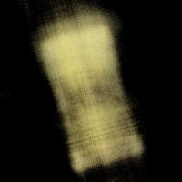
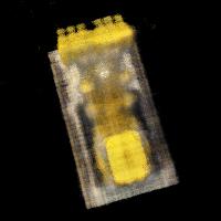
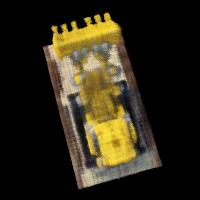
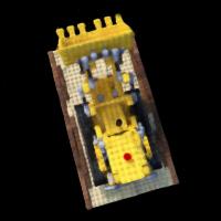
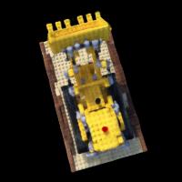
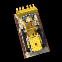
We can also make a gif showing how the image becomes more clear:

Similar to part 1, we can also compute PSNR curves, this time on our validation set:
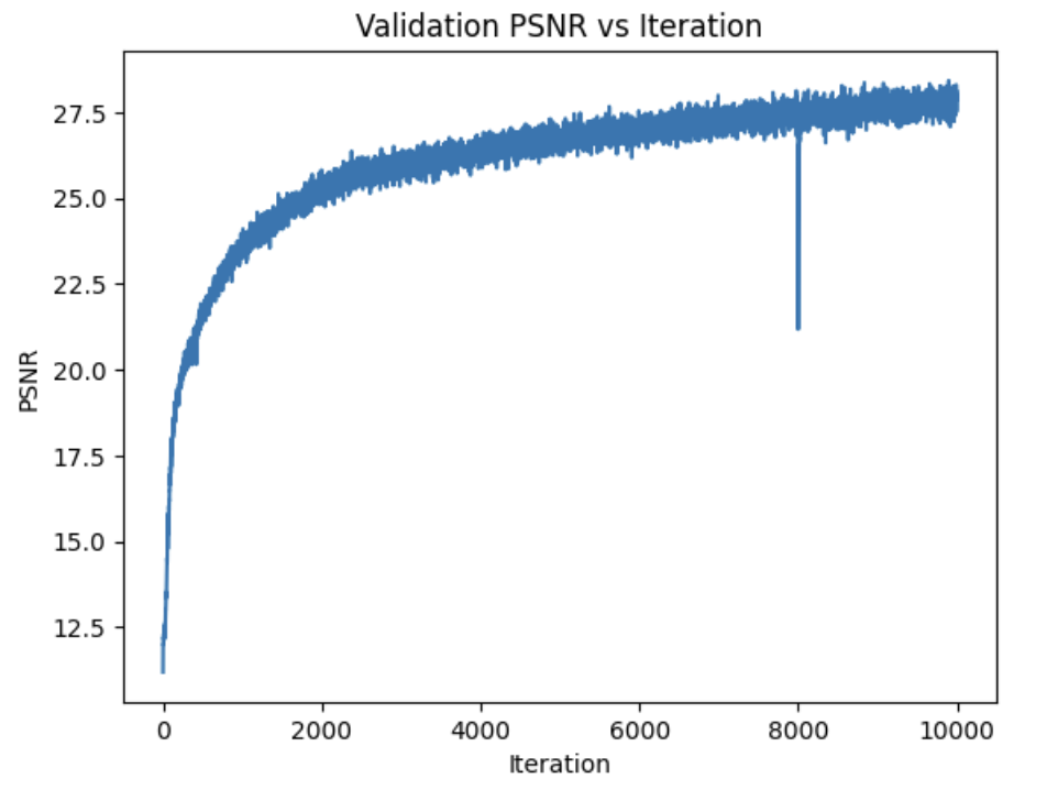
The small spike at 8K occured because after training for 8K iterations, I added an additional 2K training steps, which for some reason resulted in a brief dip in PSNR before returning to the original trajectory.
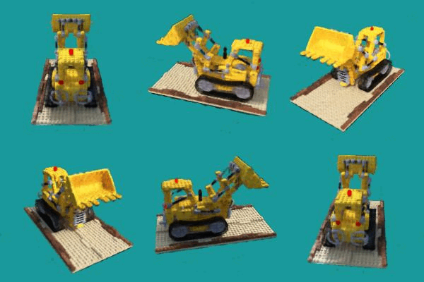
With our fully trained MLP and pixel prediction pipeline, we can now generate novel views, such as from the test set. Using only the focal length, the given c2w matrix of the test set camera location + direction, and every pixel coordinate in the 200x200 images, we can predict pixel values. This results in a pretty cool simulated lego set from 360 angles:
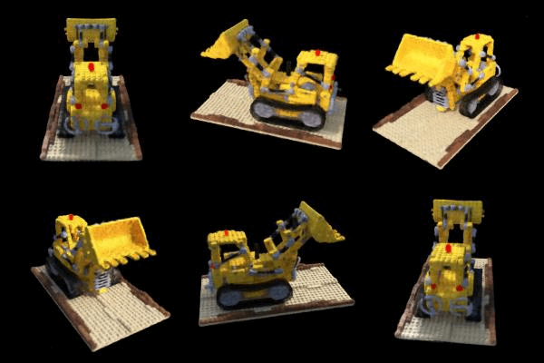
By slightly altering the color rendering equation, we can inject background colors into our simulated views, instead of a blank black background.
In the original equation $T_i$ represents the probability of a ray not terminating before our sample location $i$, and $1 - \exp(-\sigma_i \delta_i)$ represents the probability the ray terminates, or gets reflected/absorbed at location $i$, thus influencing the color on our imaging plane. The background color occurs when this ray never stops along our samples, with probability $\prod_{i = 1}^N T_i$. Typically, in this case the "color" reflected back is $(0, 0, 0)$, ie. black. But instead, we can change our equation to add a different color reflected back in the case where the ray never terminates.
In equation form, we can change our equation to be: $$\hat C(\mathbf{r}) = \mathbf{c}_b \prod_{i = 1}^N T_i + \sum_{i = 1}^N T_i (1 - \exp(-\sigma_i \delta_i)) \mathbf{c}_i$$ Where $\mathbf{c}_b$ is our set background color. So we reflect back the background color weighted by the probability the ray never ceases.
Implementing this in code allows us to change the background from gray to teal:
