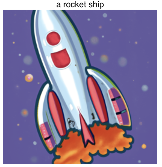
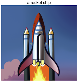
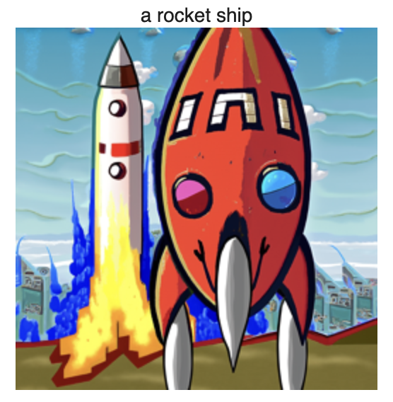
During this part of the project, we experiemented with pre-trained diffusion models, more specifically the DeepFloyd IF diffusion model and its denoisers.
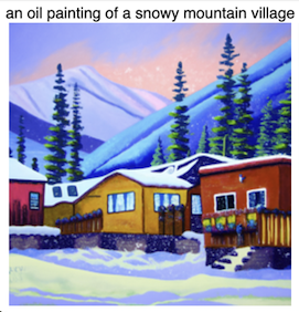
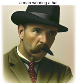
To begin the project, we generate three images using DeepFloyd's two stages using different numbers of inference steps, just to get an idea for the quality of outputs we might expected from DeepFloyd, and how the number of inference steps affects quality. For reproducibility, for the entire first section of the project we use random seed 42.


In general, it seemed more detailed prompts gave better results. In my opinion, the toil painting looks best, while the rocket ship looks worst, which makes sense given the detail given to prompt the oil painting (painting style, specifically oil painting style), and the lack of detail given to the rocket prompt. Also the number of inference steps didn't necessarily increase how good the rocket looked, but added a lot of complexity to the image: more details, background, etc.
After trying out the out-of-the-box DeepFloyd model, we specifically looked at the U-net denoising model that DeepFloyd depends on.
To begin, I implemeted the forward process of diffusion, where we gradually add noise to a clean image. The amount of noise is dictated by noise coefficients provided by DeepFloyd:
$$ x_t = \sqrt{\bar \alpha_t} x_0 + \sqrt{1 - \bar \alpha_t} \epsilon \quad \text{where } \epsilon \sim N(0, I) $$ Where $x_t$ is the noised image at timestep $t$, $x_0$ is the clean image, $\bar \alpha_t$ is the noise coefficient for timestep $t$, and $\epsilon$ is random noise.
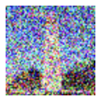
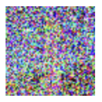
Below are some examples of the noising process for a test image over T = 1000 iterations.

Having generated our noisy images, we can start playing around with different ways of denoising them. Earlier in the class we learned about using a Gaussian low pass filter to denoise images. Before using any of the fancier denoisers, we can give the Gaussian blur a try:


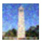


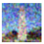


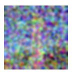
Evidently, the performance is not very strong.
Now, we can try directly passing the noisy image through DeepFloyd's pretrained U-net denoiser.


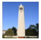


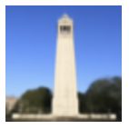


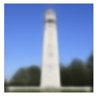
Evidently the performance is significantly better, but at higher noise levels, the original image tends to be somewhat lost.
In practice, diffusion models denoise iteratively rather than in one shot. To speed things up and save on computation, we use a strided iterative denoising process, where instead of denoising through all $T = 1000$ timesteps, we can skip a few steps by defining a new set of "strided" timesteps that correspond to certain intermediate noisy images.
Then, when updating from the $t$th image in the strided set to the next image (slightly more clean): the $t'$th image, we can use the following formula: $$ x_{t'} = \frac{\sqrt{\hat \alpha_{t'}} \beta_t}{1 - \hat \alpha_t} x_0 + \frac{\sqrt{\alpha_t} (1 - \bar \alpha_{t'})}{1 - \bar \alpha_t} x_t + v_\sigma $$ Where $\alpha_t = \frac{\bar \alpha_t}{\bar \alpha_{t'}}$, $\beta_t = 1 - \alpha_t$, and $v_\sigma$ is some random noise. The rest of the variables are the same as they were in the previous equation in the forward process.
Implementing the iterative process gives us the following results:
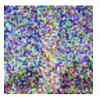
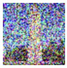
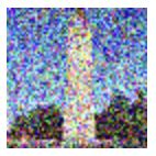
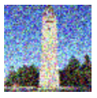
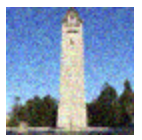
Comparing each of the denoising methods:

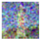
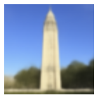
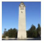
It seems clear that iterative denoising performed the best (starting from the noisy image at $t = 990$)
Our iterative denoiser also can work as an image generator; we just pass in truly random noise, conditioned on the prompt "A high quality image". Here are five sample images from this process:
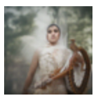
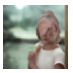
Some of these images look decent, like sample 5, but generally they aren't great in quality.
To improve the images, we can use a technique called Classifier-Free Guidance, where we generate both a conditional and unconditional noise estimate, and use the two of them to generate a final noise estimate using the formula: $$\epsilon = \epsilon_u + \gamma (\epsilon_c - \epsilon_u)$$ And setting $\gamma$ to be greater than 1, in which case we skew our noise estimate to the difference beweetn the conditioned and unconditioned noise estimate. The concept seems pretty similar to the caricutures idea in a previous project.
Using Classifier-Free Guidance with our iterative denoiser, we can produce some better quality photos:

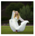

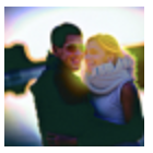
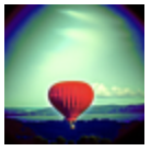
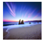
Now that we have our cfg-iterative denoiser, we can do some pretty neat things with it, such as editing a photo. The idea is to add some noise to the original photo using our forward process, then denoise the noisy photo to get a new photo. The more noise we add, the less the end photo will resemble our original photo at all. Here are a few examples:

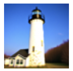
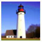
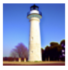
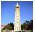



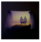




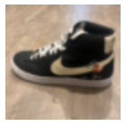
The above process is more interesting when applied to non-realistic photos, such as drawings or cartoons pulled from the web. In both cases, in theory the edit could make the original image more realistic.
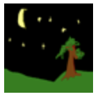


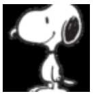

We can also mask out a certain section of an image, and have the diffusion model denoise that section only, while coercing all other pixels to return to their original values.
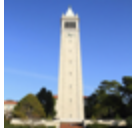





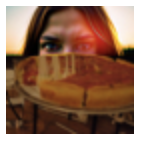
We can also condition our diffusion model on different natural language prompts (up to this point we had been conditioning on "A high quality image"). Below are some examples, where the lower photos have less noise added and the higher photos have more noise added.


One of the more cool things we can do is to create illusions where an image appears to be one thing when rightside up, but turns into a completely different thing when flipped upside down.
To have our diffusion model create these images, at each time step we essentially predict the noise of the image conditioned on one text prompt, flip the image, and predict the noise condition on the other text prompt. These two noises are then combined for our final noise estimate to be used for denoising. $$ \begin{aligned} \epsilon_1 &= \text{UNet}(x_t, t, p_1)\\ \epsilon_2 &= \text{flip}(\text{UNet}(\text{flip}(x_t), t, p_1))\\ \epsilon &= (\epsilon_1 + \epsilon_2)/2 \end{aligned} $$ Below are some examples of visual anagrams we can create:
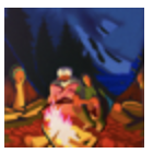


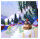
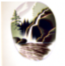
In a similar vein to the previous part, we can create images that look like one thing from close up, and another from far away (or blurring your eyes)
To achieve this, we generate two noise estimates, each conditioned on a prompt. The noise estimate corresponding to the prompt we want to see from close up, we high pass. The noise estimate corresponding to the prompt we want to see from far away, we low pass. Then we just add the noises together for our final noise estimate. Here are some examples:
In the previous section, we used a pre-trained DeepFloyd model. In this section, we build and train our own U-Net, specifically trained on the MNIST dataset of handwritten numbers.
We begin by building up a simple U-Net architecture as outlined in the project spec. The model learns kernels such that it can denoise an image into a digit by taking the 1x28x28 image in, creating many hidden layers (for this first part we use 128), and pass the transformed image through various layers of dowmsampling, upsampling, and convolutional blocks (plus some skip connections using tensor concatenation)
To train this U-net, we need noisy images, which we can generate using Gaussian noise: $z = x + \sigma \epsilon$ where $\epsilon$ is our Gaussian noise, and $\sigma$ controls the strength of the noise. Below are a few different noise levels visualized:
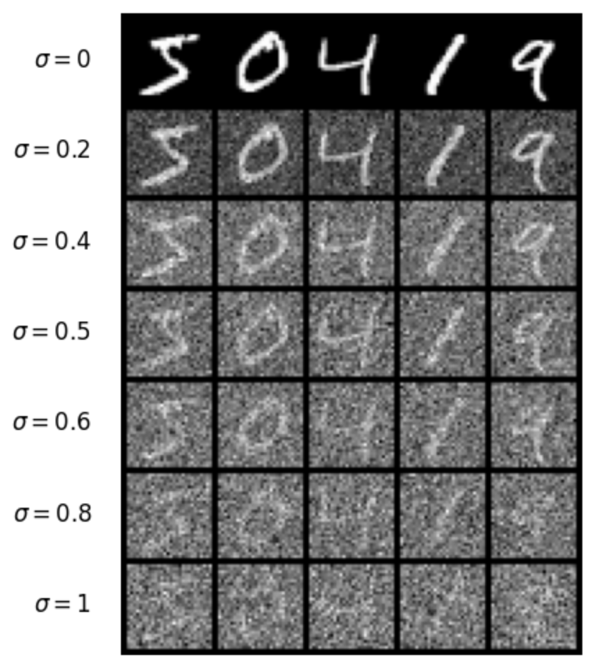
We choose to work with $\sigma = 0.5$ and train the U-net on our MNIST dataset using hidden dimension $D = 128$, and an Adam optimizer with learning rate $1e-4$. Over 5 epochs, here is the training loss plot:
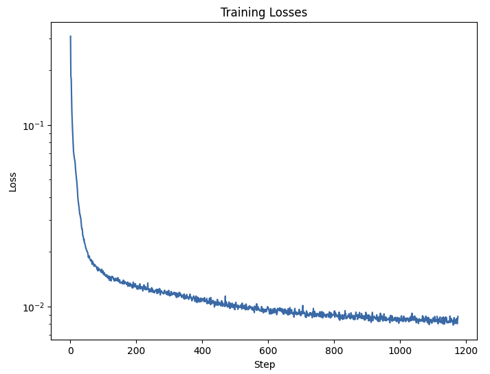
And below we can see the results of applying the U-Net after 1 epoch of training, and 5 epochs of training.
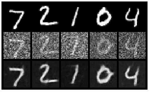
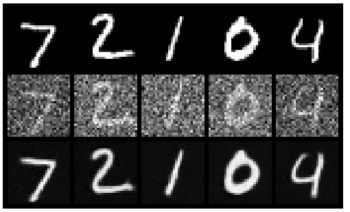
The U-Net was only trained on the specific cases where the noise added had parameter $\sigma = 0.5$. So we can test it on out-of-distribution examples at various other $\sigma$ levels:

Now that we have a basic U-Net, we can use it to create a diffusion model.
From the previous parts of the project, we know that a one-shot diffusion model is less effective than a iterative diffusion model. That means we need to introduce some dependency on $t$ the denoising step, into the U-Net.
We do so by introducing two FCBlocks that take in $t$ as an input and are added to blocks during our upsampling stage.
We also need a set of noise coefficients, which are derived based on the procedures in the project spec. Finally, our loss is defined as the MSE of our predicted noise vs. the actual noise. Implementing these changes and training the U-Net, we get the following training loss curve:
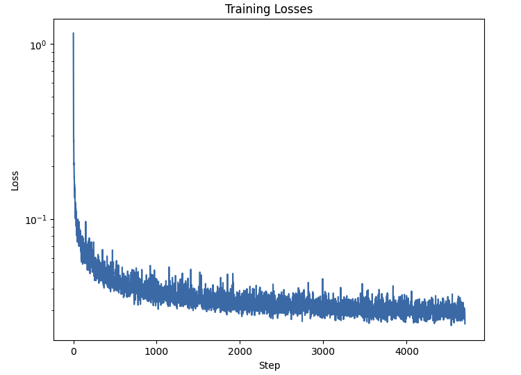
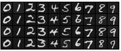
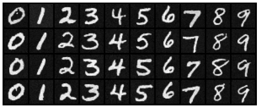
We also define a sampling procedure which is similar to our previous parts, but we replace the added variance with $\sqrt{\beta_t}$. Using this sampler, we can produce the following digits after 5 and 20 epochs.
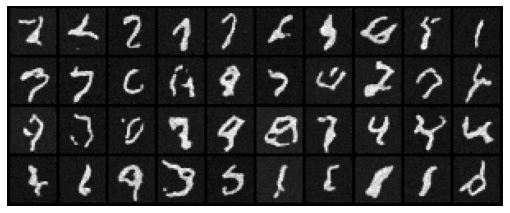
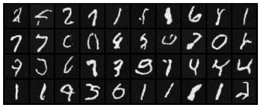
Clearly, the digits from the previous section weren't great. To improve the performance of our U-Net, we can condition on class, ie. the kind of digit we are generating. Since there are exactly 10 possible digits, we can pass in a length 10 one-hot encoded vector to our U-Net, essentially allowing it to learn to denoise different for each digit.
To do so, we add two more FCBlocks into our architecture, which take the one hot encoded vector and produces a tensor to multiply into existing blocks during our upsampling stage, essentially conditioning the output on the class of digit we manually pass in.
For both the training and the sampling procedure, we also have a probability of dropout, where 10% of the time, we pass in a zero vector instead of a one-hot encoded vector, essentially getting rid of conditioning for that specific iteration/training pass.
These modifications result in the following training loss plot:
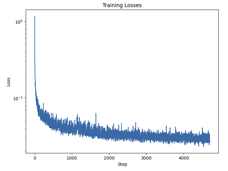
And now after 5 and 20 epochs, we get significantly better digits!
