In the first section of this project, we were tasked with recovering homographies from one image to another based on manually defined correspondence points, then using these homographies to both rectify and stitch together Mosaics of different images.
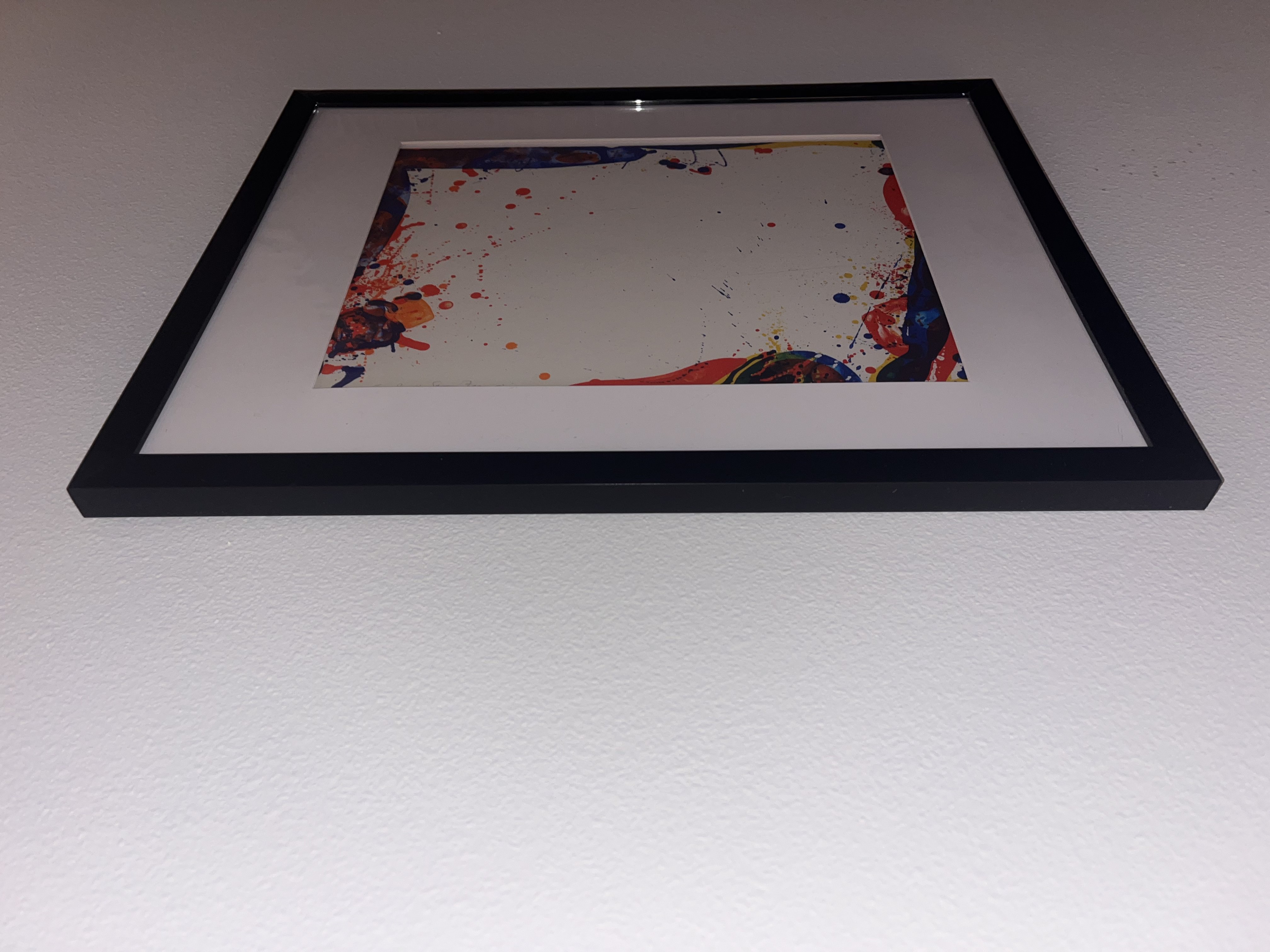
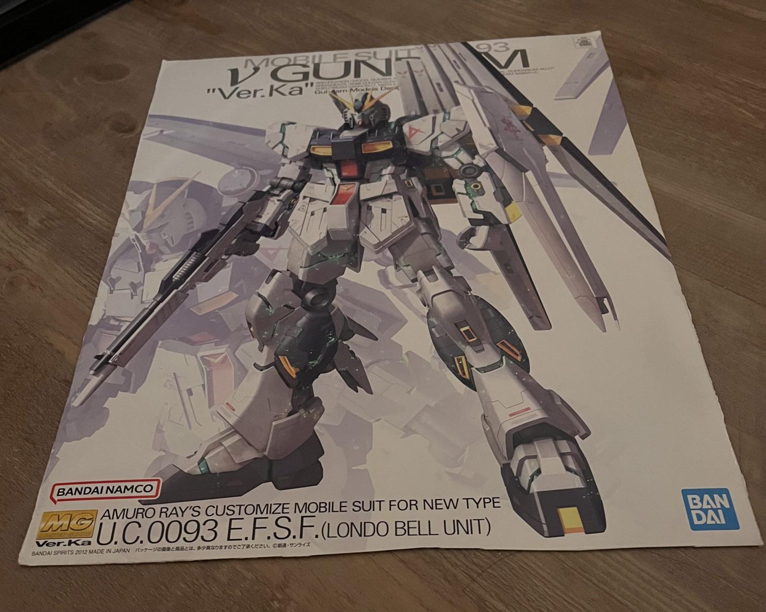
Below are the images I used for the rectification portion of the project:


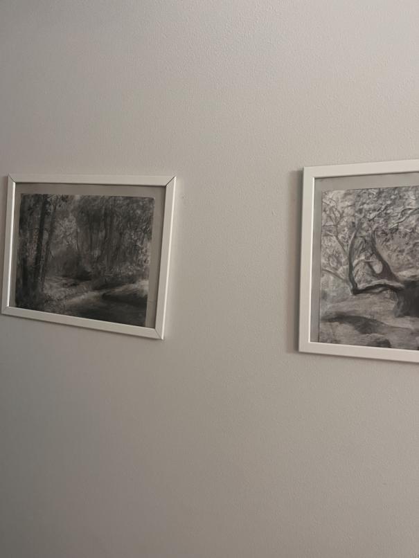
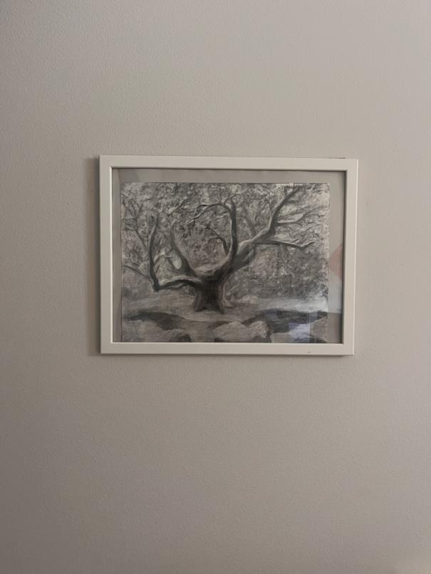
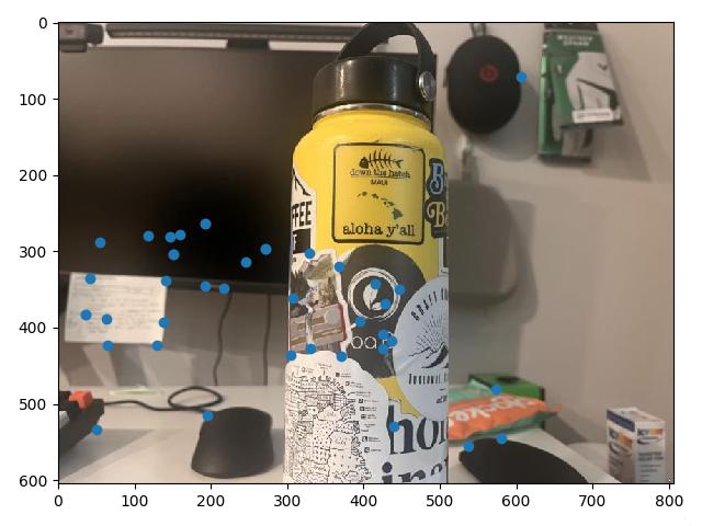
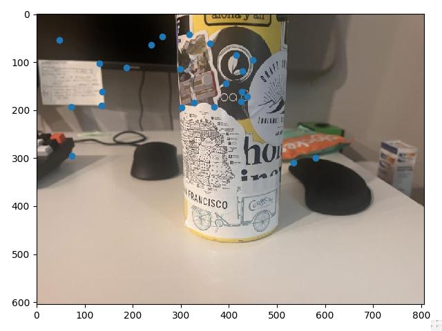
And here are the images I used for the mosaicing portion of the project:
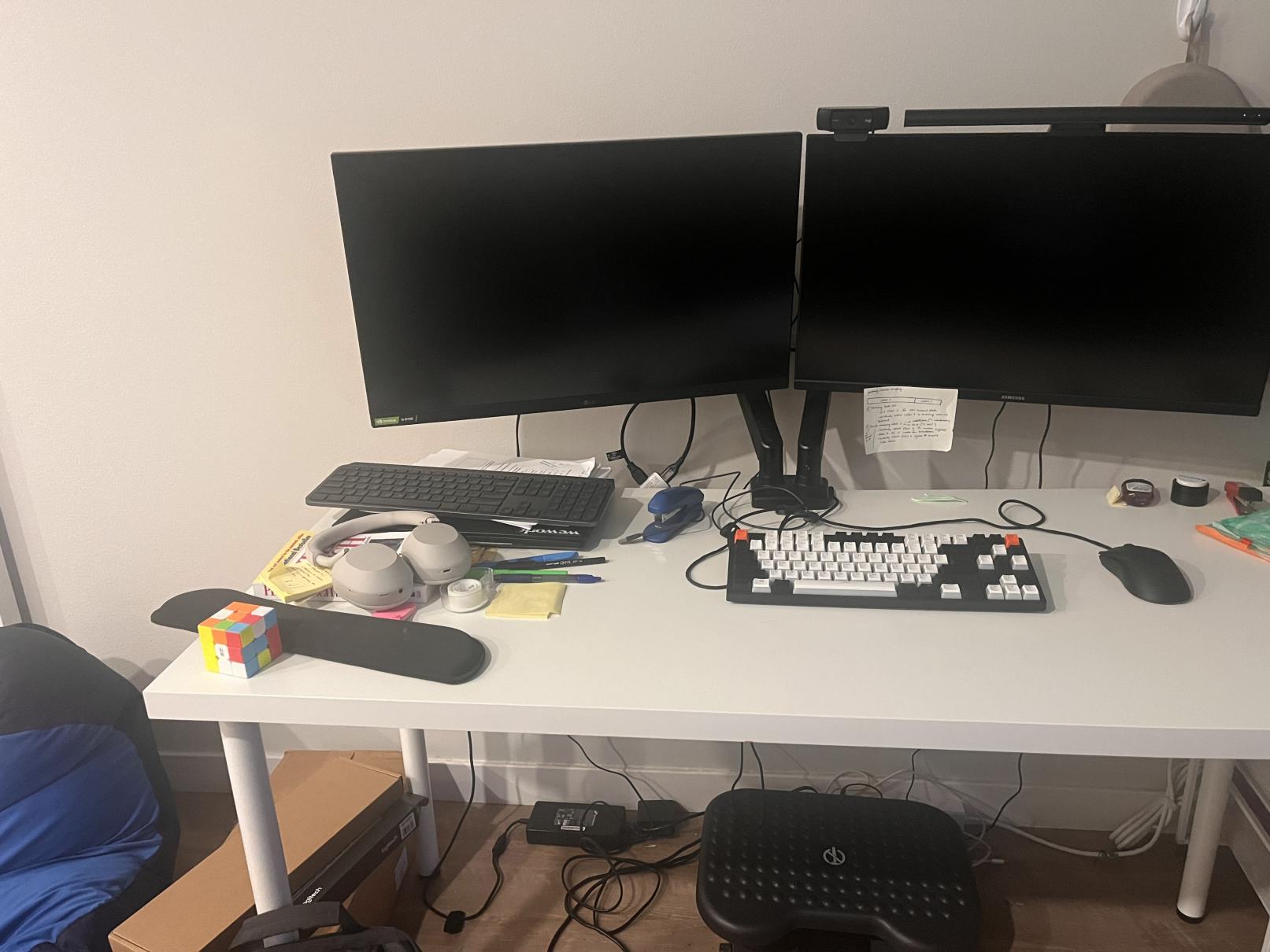
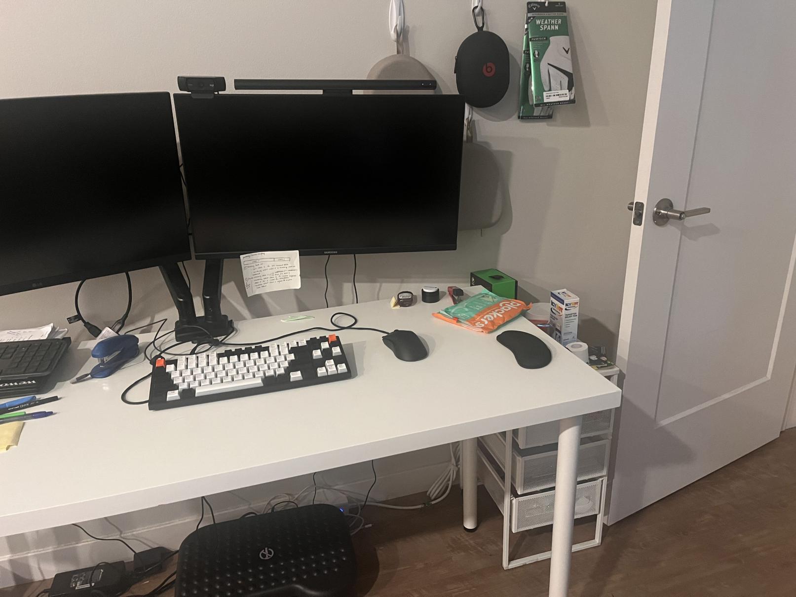
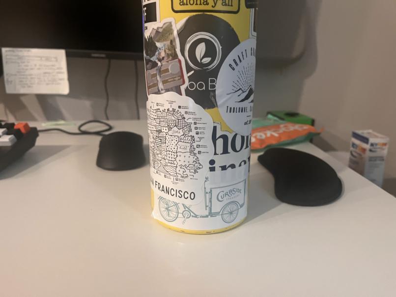
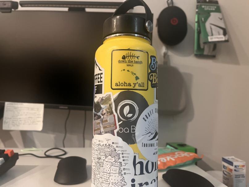
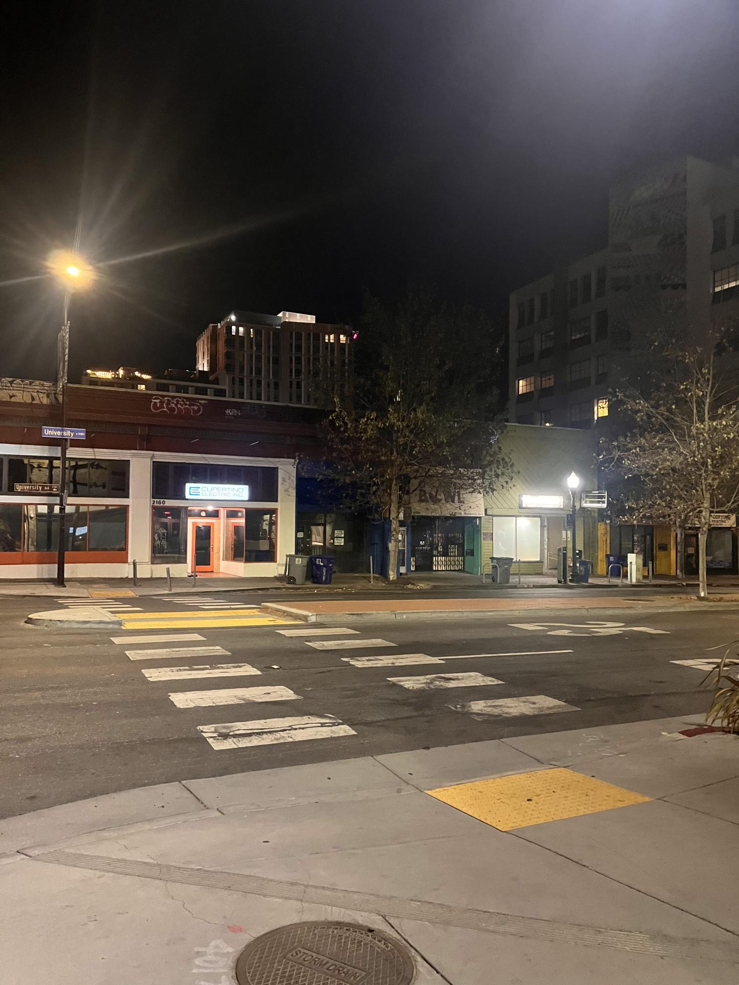
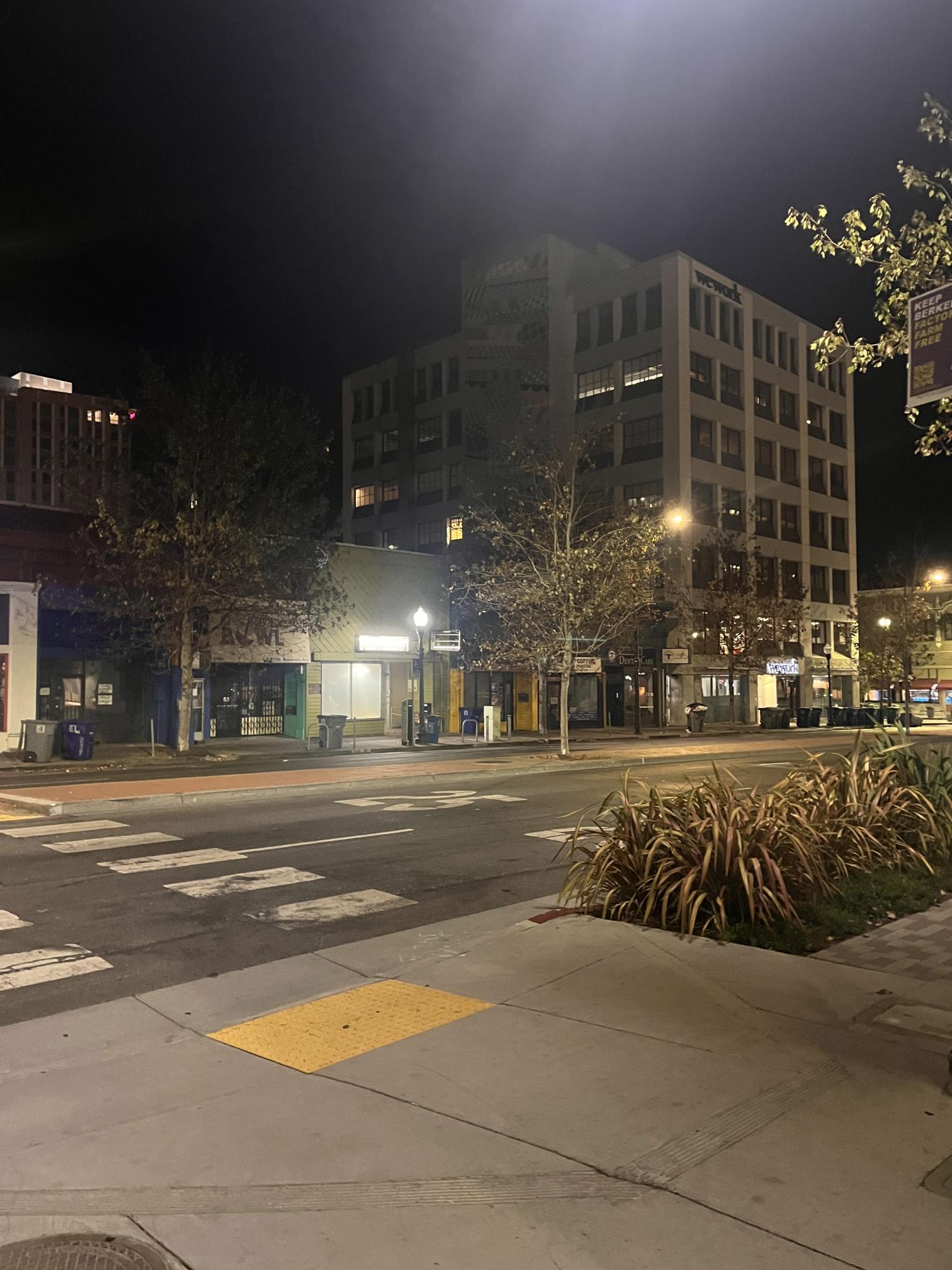
The first step in both rectification and in mosaicing is recovering homographies. To do so we define several correspondence points manually, for this I used a provided correspondence tool.
Our goal is to find a 3x3 matrix of the form: $$ H = \begin{pmatrix} a & b & c \\ d & e & f \\ g & h & 1 \end{pmatrix} $$ Such that for each correspondence point the following holds: $$ H \begin{pmatrix} x \\ y \\ 1 \end{pmatrix} = \begin{pmatrix} wx' \\ wy' \\ w \end{pmatrix} $$ Where $x, y$ are the coordinates of the starting point, $x', y'$ are the coordinates of the ending point, and $w$ is some scaling factor (which we will divide out to find the true projected coordinates).
Then, for each point we can expand out the above condition:
$$
\begin{cases}
ax + by + c = wx' \\
dx + ey + f = wy' \\
gx + hy + 1 = w \\
\end{cases}
$$
Then, substituting $w = gx + hy + 1$, we get:
$$
\begin{aligned}
\begin{cases}
ax + by + c = (gx + hy + 1)x' \\
dx + ey + f = (gx + hy + 1)y' \\
\end{cases}\\
\begin{cases}
ax + by + c = gxx' + hyx' + x' \\
dx + ey + f = gxy' + hyy' + y' \\
\end{cases}\\
\begin{cases}
ax + by + c - gxx' - hyx' = x' \\
dx + ey + f - gxy' - hyy' = y' \\
\end{cases}
\end{aligned}
$$
Since we know $x, y, x', y'$ for each correspondence, our task is to find values for $a$ to $h$. Since we'll have many correspondences (at least 4 to make the system solvable), we cannot get an exact solution, but we can use
least squares to get an approximate solution.
We can then use numpy.linalg.lstsq to approximate the homography matrix after rewriting the above equations in matrix form, and stacking the matrices for correspondences.
To warp images using homographies, we use a similar process to project 3. After defining the corners of the image we are warping, we can apply the homography matrix to those corners to retreive the corners of the warped image. These warped coordinates are often negative, which is an invalid index for an array representation of the image, so we end up needing to shift the corners appropriately.
Obtaining the corners of the warped image allow us to use skimage.draw.polygon to retrieve all of the discrete points within the warped image. We can then use an inverse warp to fill out the pixel values for each of the points within
the final polygon. More specifically, we compute the inverse of the homography matrix, map points in the warped image back to locations in the original image (being sure to account for $w$!), then interpolate pixel values since the inverse warped location
may lie between pixels.
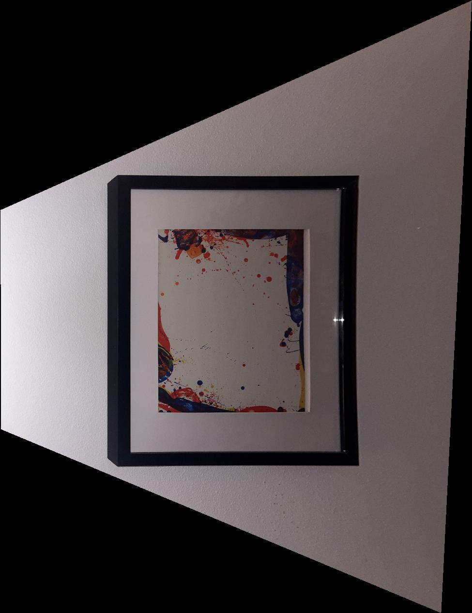
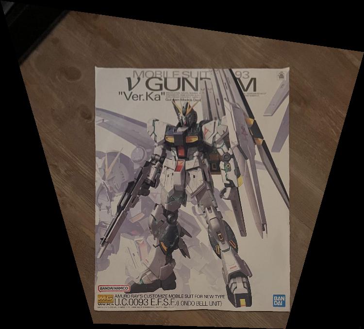
The above generally outlines the warp procedure. After implmenting it, we're ready to rectify.
To rectify an image, we manually define correspondences between the original image (specifically the corners of whatever we want to rectify) and a rectangle we manually define. The results are shown below:


The final step of the first major section of this project was to mosaic images together. The images for mosaicing shown above were taking from one constant location, changing the viewing angle between images, while leaving overlap. The overlap allowed me to define correspondences between points in the two images (points that were on top of the same visual object but were different in pixel locations because of the viewing angle change).
After defining these correspondences, warping one image to the other using the above method on warping would match up the correspondences as best as the homography could. The only added consideration was the shifts. Since sometimes we would need to shift the first image to prevent negative coordinates, the second image would need to be shifted as well.
Warping and shifting completed, we have two images which overlay well structurally, but need to be blended. I implemented two different blending techniques. The first was a linear gradient blend, where the overlapping regions between the two images after warping had either a horizontal or vertical gradient for $\alpha$ values, ie. for pixels that were only represented by image 1, $\alpha = 1$, for pixels that were only represented by image 2, $\alpha = $0, but in the overlapping region, images to the left/top would have a greater $\alpha$ value, and gradually move to $0$ as they moved right/down.
The other blending technique was a two band blend. In this method, each image is broken into a high pass and low pass image. The high pass images are blended using a hard blend, and the low pass images are blended more "smoothly".
More specifically, we defined a distance transform for image 1 and another for image 2. These are arrays of the same shape as the images, where each element represents the distance the corresponding element/pixel of the image to a "background pixel", or a pixel of value 0. This has the effect of creating a mask that has high values within the center of the polygon representing the warped image, and gradually lower values as you get closer to the edge of the polygon
We use these distance transforms (after normalization) as $\alpha$ weights when blending the low passed images. For the high passed images, we defined a mask by the maximum value of the distance transforms. If at a certain pixel, the distance transform for image 1 has a higher value than the distance transform for image 2, in the high pass blend we will take the pixel from image 1. The same holds in reverse if the distance transform for image 2 is greater.
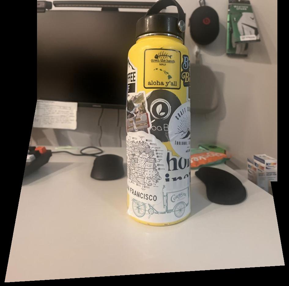
The final thing of note is that before the entire process of blending, we would erode the masks representing the locations of each warped image within the entire array. This is because without erosion, the Gaussian blur ends up picking up on noise from the background pixels, leading to strange dark artifacts in the final blend. The results of each mosaicing + each blending technique are shown below.
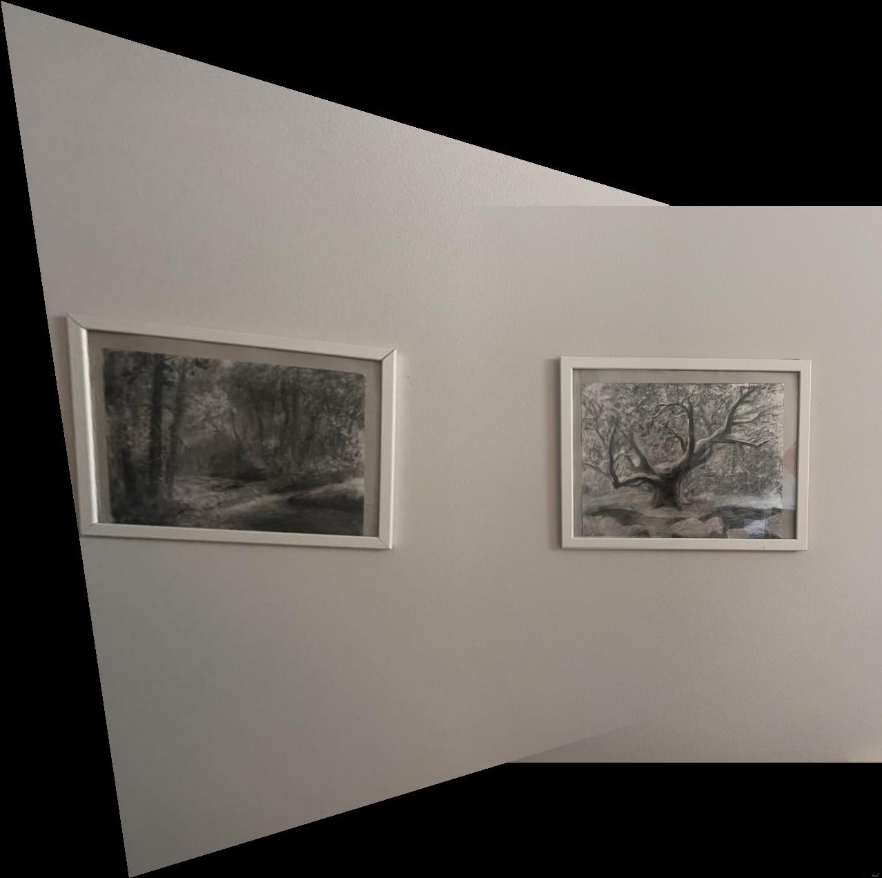
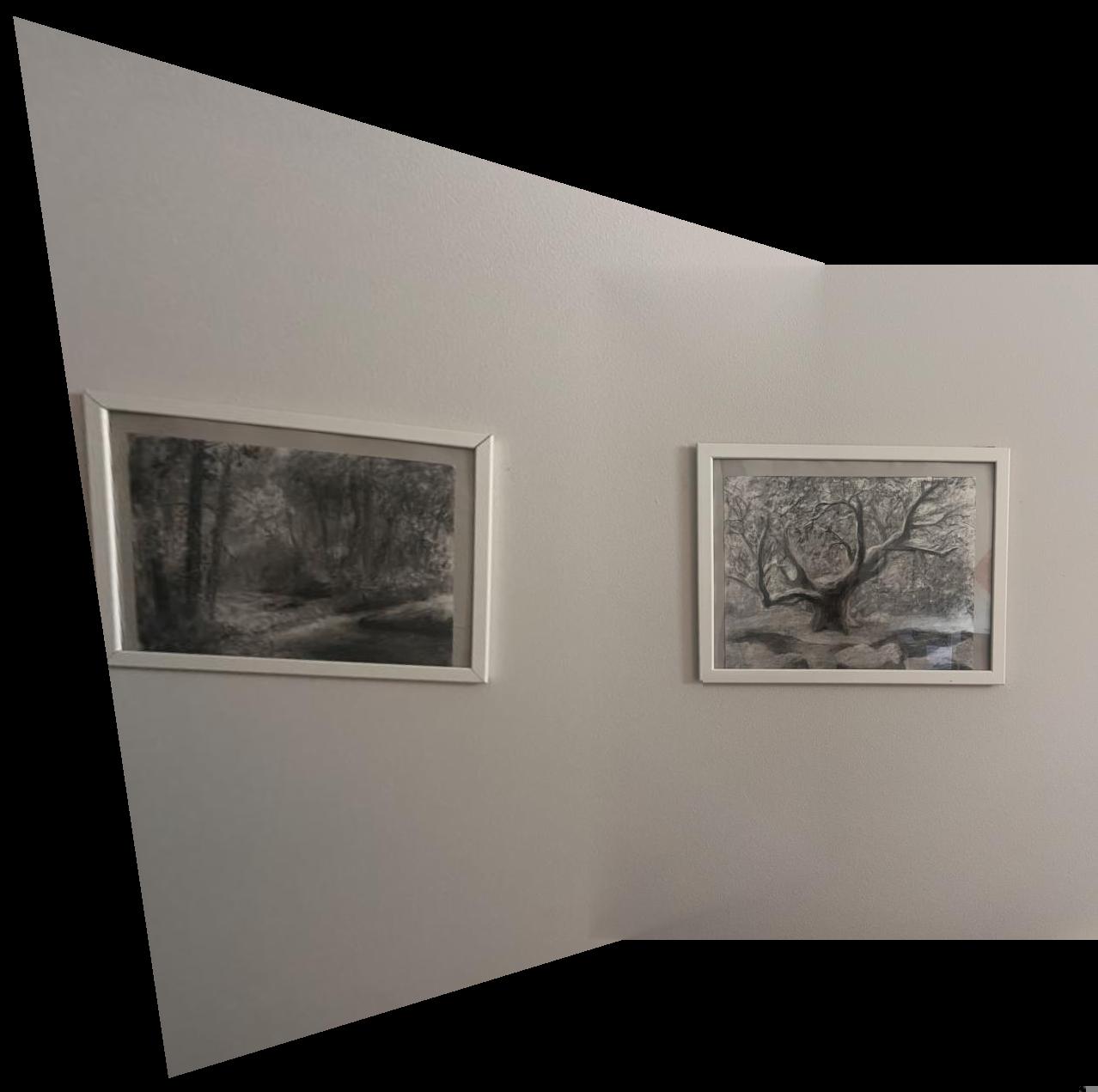
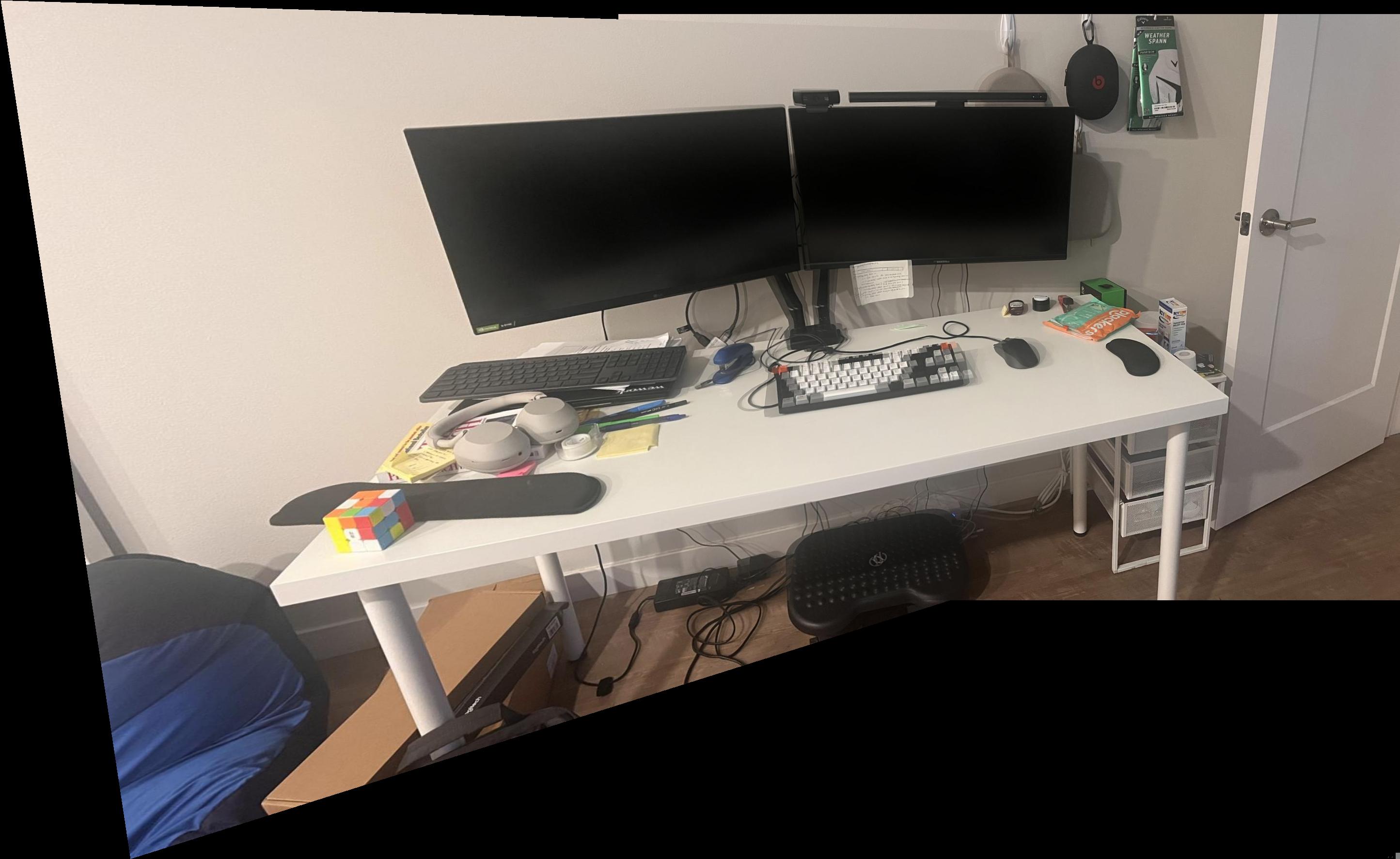
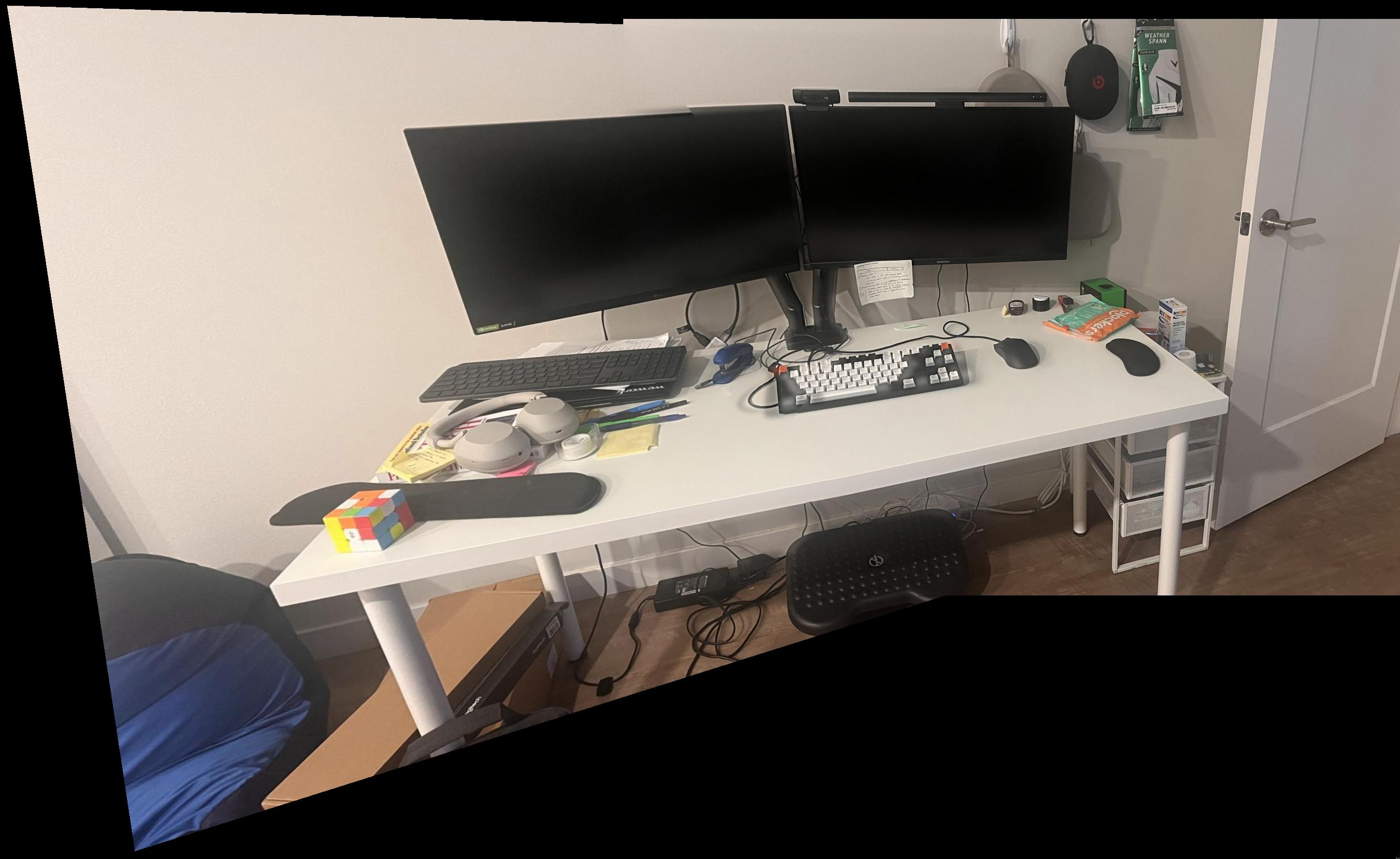
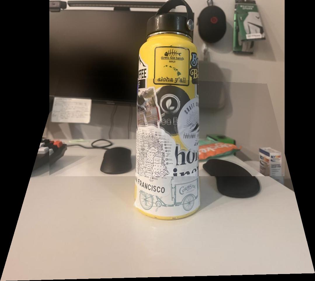
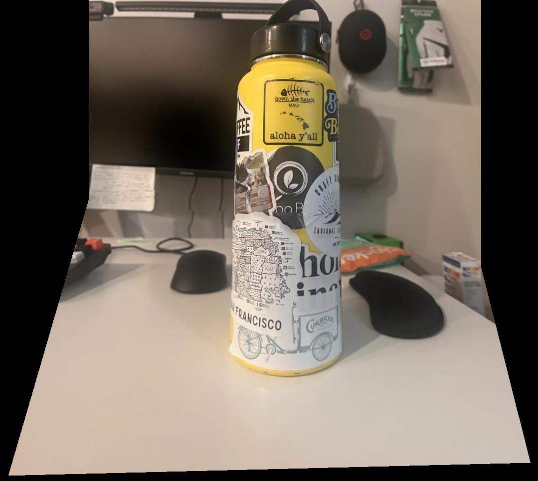
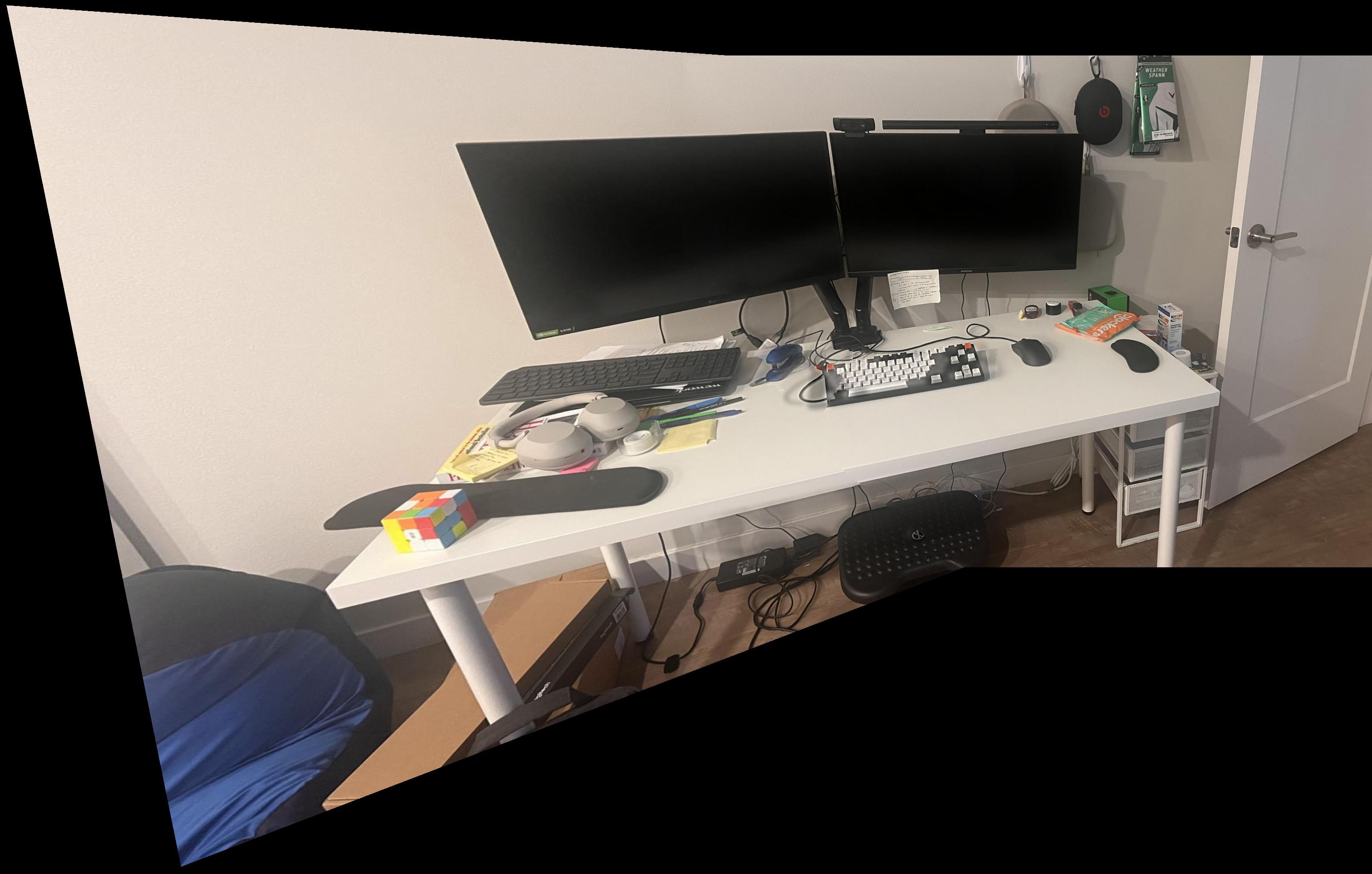
Both blending techniques ended up having some artifacts. The hanging image seemed to perform better with the linear blend, likely because the linear blend is extremely effective on uncomplicated backgrounds. However, for a more complicated mosaic, the two band ended up having the best effect, though there are still some artifacts (top of the left computer screen in the desk example, and the cut off text on some stickers in the water bottle example).
In this section, we implement methods which allow us to automatically define correspondence points, rather than point and click correspondences between two images. The process will be illustrated on the images of University Ave, and at the end the images for the other mosaics will also be shown.
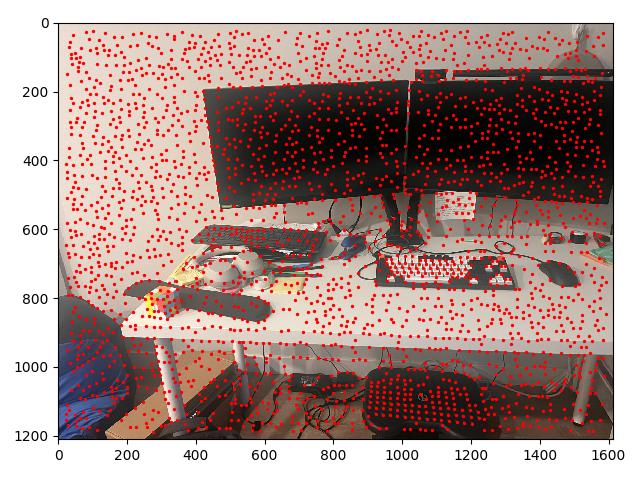
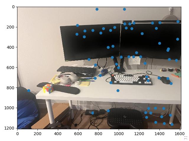
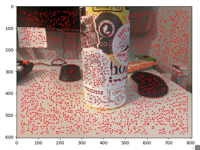
To begin, we use a Harris edge detector to find potential points of interest. Using the provided code, and appropriately setting the min_distance parameter to limit the number of
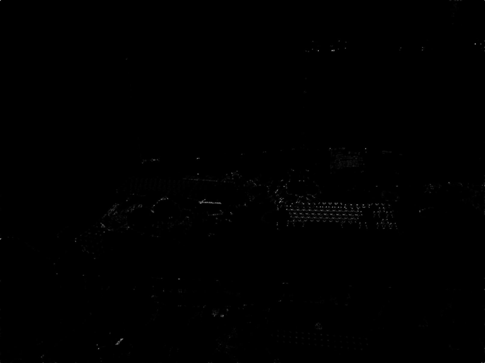
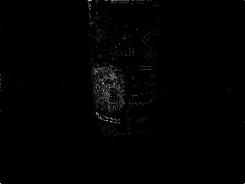
identified points to around 2000, we create a set of interest points at which we may potentially form correspondences, along with a matrix that represents the corner strength of every point in the image.
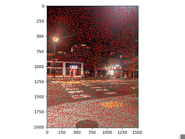
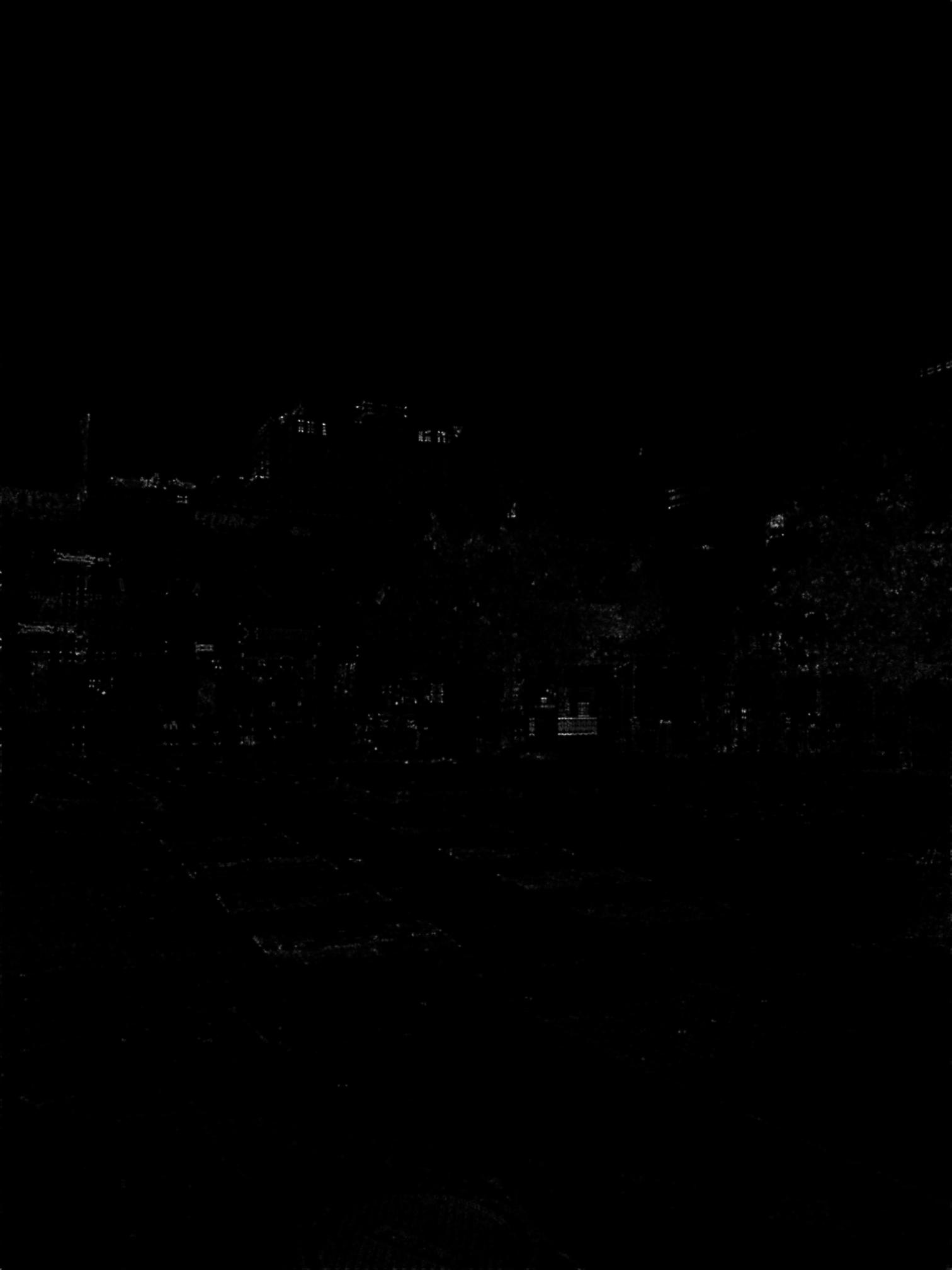
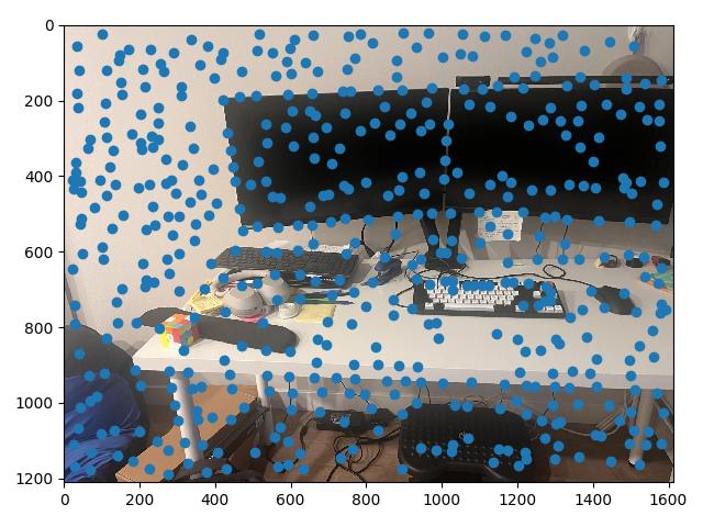
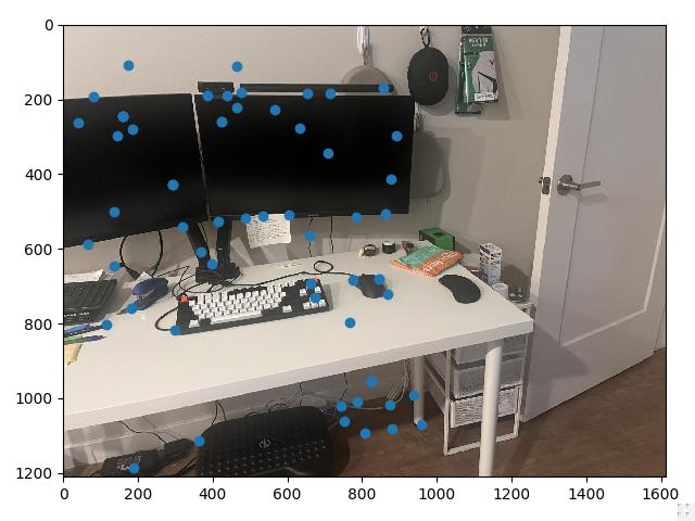
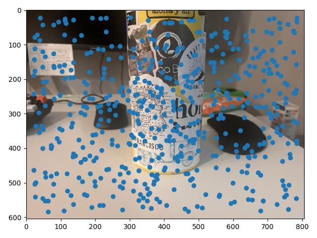
Harris points give us a good start, but provide a lot of corners, many of which are not particularly "high quality" corners that correspond visually to some real object. To find a stronger subset of these corners, we can use a simplified version of a technique from Multi-Image Matching using Multi-Scale Oriented Patches, called adaptive non-maximal suppression, or ANMS. The main idea is to define some radius $r$, and at each Harris point evaluate whether or not that point is has the maximum corner strength value within a circle with that radius.
The paper also points out a different way of observing this problem, rather than setting a radius and finding the maximums, we can find the largest radius value for each Harris point such that it remains the maximum within that circle. This radius value corresponds to the largest $r$ we could chooose and still have the point remain unsuppressed.
This radius is also defined by the closest neighbor to our point of interest that has a larger corner strength value than our point of interest, since exactly when that neighbor is within the bounds of the circle, our point of interest ceases to be a local maxima and is suppressed. This special radius value is dubbed the "minimum suppression radius" by the authors, and is formally defined for each point indexed by $i$ as: $$r_i = \min |x_i - x_j|, \text{ s.t } f(x_i) < c f(x_j), x_j \in \mathcal{I}$$ Where $|x_i - x_j|$ represents the distance between $x_i$ and $x_j$, $f(\cdot)$ is the corner strength function, and $\mathcal{I}$ is the set of all Harris points. $c$ is an additional parameter that controls the robust-ness of the suppression, by setting $c$ to be a lower value, we force features to be a decent amount smaller than its neighbor for that neighbor to set the radius value.
These radii then also rank the order in which each point is added to our unsuppressed set as $r$ decreases from infinity. At $r = \infty$, only the global maximum is included. As we decrease $r$, we "add" new points which are local minima within radius $r$. So finding the $n$ points with the $n$ greatest $r_i$ values is equivalent to automatically setting an $r$ value to retrieve $n$ points.
Long story short, instead of testing out different $r$ values, we can actually just specify how many points we'd like to suppress to, which is convenient!
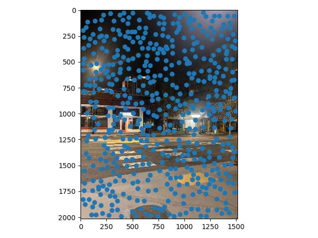

Now that we have a set of points that we reasonably believe can represent real visual features, we would like to describe each one of them (so we can match points between our stitched images later). To do so, we take 40x40 axis-aligned chunks around each unsuppressed point, apply a Gaussian filter (to prevent aliasing), and downsample the chunk to an 8x8 pixel chunk. This chunk, when flattened to a length 64 vector and normalized to mean 0, std 1, is our feature vector for that point, representing the general visual information surrounding that point.

After creating features for all $n$ points we have after ANMS on both images we are trying to find correspondences for, we can begin matching features between images. To do so, we make use of Lowe's trick. We first calculate the pairwise L2 distances between all possible combinations of features from image 1 and features from image 2. Each point on image 1 has a nearest neighbor on image 2, this is our potential match. However, we want this match to be significant, and to check this we look at the second nearest neighbor of the point of interest. If this distance is also small, then we can't be certain our original potential match is actually correct, and so we throw it out.
In practice, we compute the ratio between the nearest neighbor distance and the second nearest neighbor distance, and if that ratio is less than our threshold (ie. the distance to the nearest neighbor is a good amount shorter than the distance to the second nearest neighbor), then we keep the match. Otherwise we throw it out. Thus, the smaller the threshold, the more strict we are on potential matches.
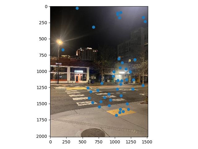
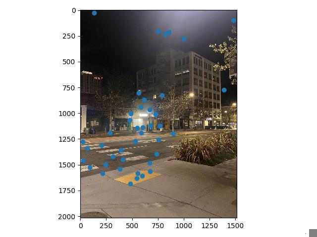
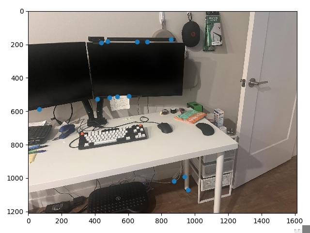
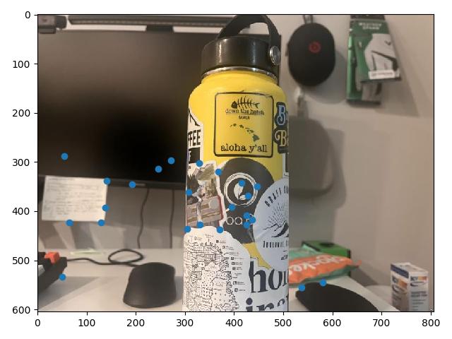
At this point, a visual inspection of the remaining feature matches shows that we have a lot of good correspondences. The issue is we still have a few points which are completely off, and would ruin any computed homography if they were included (for example, the point under the street lamp in image 1 above. The street lamp doesn't even show up in image 2.)
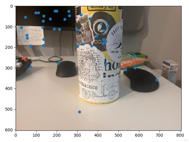
To make of feature matches fully robust, we use a Random Sample Consensus, or RANSAC. For a set number of iterations, in each iteration, we take a random sample of 4 feature matches, and use them to compute a homography from image 1 to image 2. That homography is then applied to all remaining potential matched points in image 1. This retrieves the hypothetical points our correspondences would be mapped to using this homography, and by comparing them to their actual correspondence values, we can see how well the computed homography maps all of our potential correspondences.
This allows us to create an inlier set, a set of points for which the homography warps close to the corresponding point on image 2, with a pixel distance below some threshold we manually set. Conducting this many times and tracking the largest inlier set gives a "group majority" of points which can cooperate with one another for a potential homography. This inlier set then becomes our set of final correspondences.

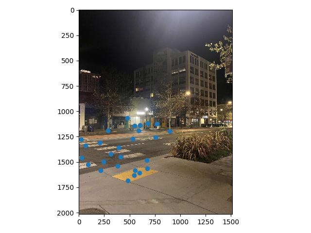
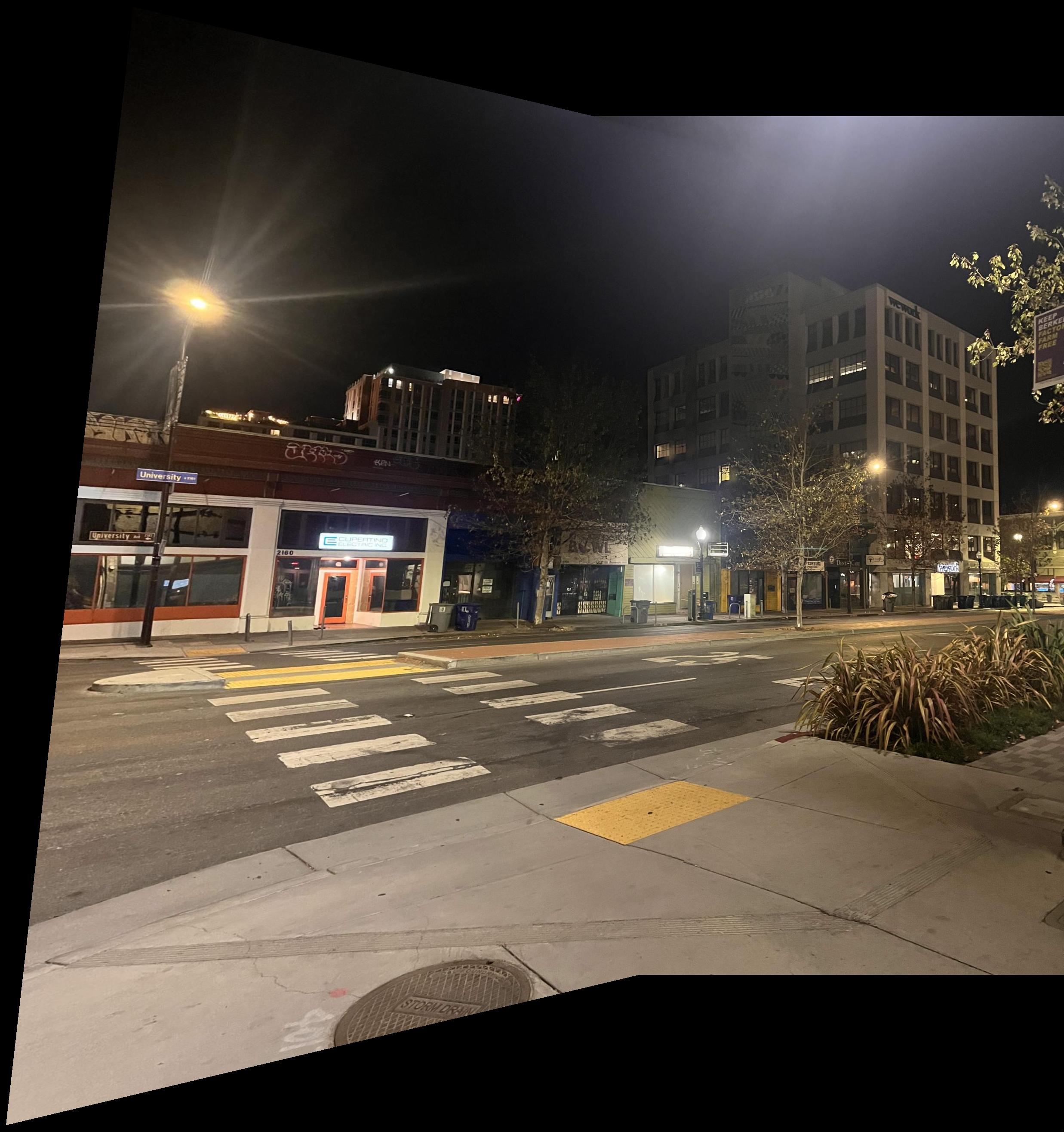
With these defined correspondences, we can use our code from Part 1 to compute a homography and blend the warped images. For the University Ave. Example, that results in the following mosaic:





The coolest thing I learned from this project was the automatic feature detection and matching portion 4B. I though the paper about ANMS was pretty interesting, especially how they explained the duality between the more conceptually simpler way of thinking about finding local maxima (set a radius first, then find maxima), and the more convenient way of thinking about it (essentially organize the points by "local strength").
I also found the whole process of seeing each step build up particularly cool. We began with Harris corner detection points, use ANMS to whittle it down to some local maxima, then use feature matching and Lowe's trick to further narrow down the possible correspondence points, and finally use RANSAC to double check those correspondences. Each step contributed a bit to my laptop being able to identify the same features using this process as I could just using my eyes to look at the images.