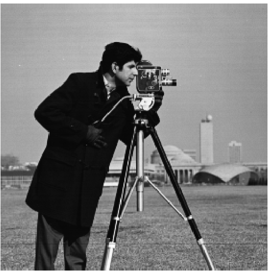
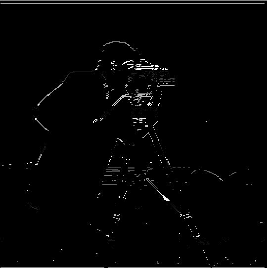
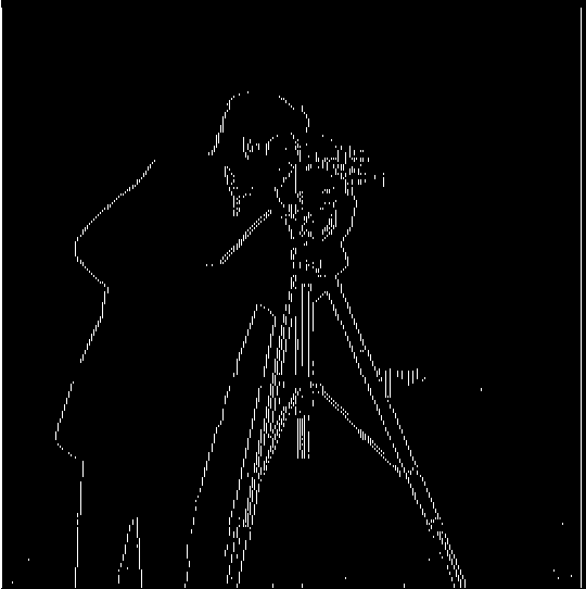
In this section of the project, use the finite difference filter to approximate the partial derivatives in the $x$ and $y$ directions. More specificially:
$$ D_x = \begin{bmatrix}1 & -1\end{bmatrix}, D_y = \begin{bmatrix}1 \\ -1\end{bmatrix} $$
We use $D_x$ and $D_y$ as filters to convolve with our image, which is intended to find large changes in pixel values in horizontal and vertical directions. To get the edges, we can take the absolute value of the partials (since negative and positive change both indicate edges) and binarize the partials using a threshold.
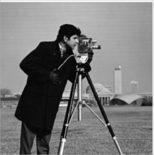
To test these filters, we convolve them on a image of a cameraman, and get the following gradients:


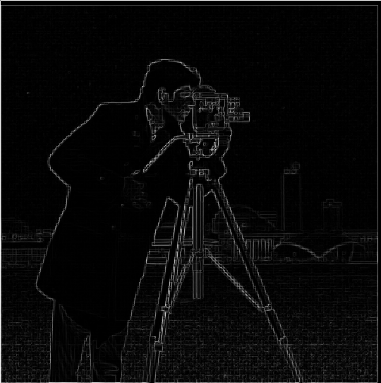
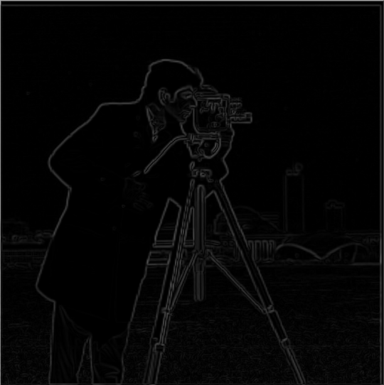
To create edges that aren't just horizontal or vertical, we can calculate the gradient magnitude, which we can calculate as:
$$||\nabla f|| = \sqrt{(\frac{\partial f}{\partial x})^2 + (\frac{\partial f}{\partial y})^2}$$
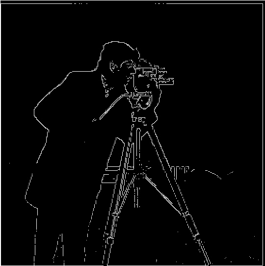
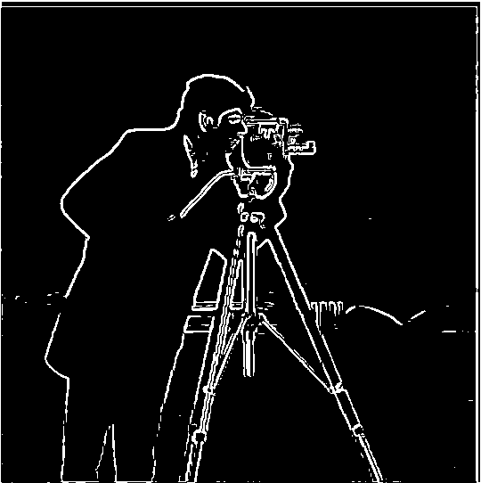
Essentially, at each pixel we take the square root of the sum of the squared x and y partial derivatives at that point, which in our case, is approximated by our convolutions. Using the above operation and our previously found partial derivative approximations, and a new threhsold, we can try and find the complete edges of the picture:
In this section, we try and sharpen images by taking the high frequency components of the image and and adding more of them to the base image. To demonstrate the process, I used the provided image of the Taj Mihal.
We first use a Gaussian filter (from the previous section) to isolate the low frequency components of the image. Then, by subtratcing this low passed image from the original base image, we can extract the high frequencies that were removed by the Gaussian filter. Finally, by adding some multiple of these high frequencies to the original image, and clipping any out of bounds pixel values, we can create a sharpened image. This is done for each channel of the image independently.

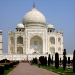
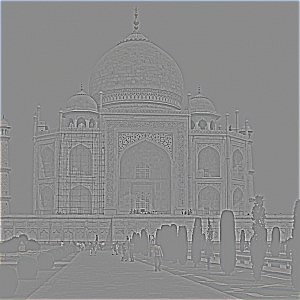
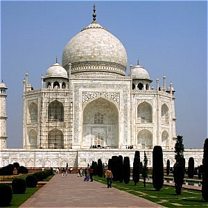
This entire process can be captured in a single convolution using the following filter: $((1 + \alpha)e - \alpha g)$, where $e$ is the unit impulse filter of the same size as the Gaussian, and $g$ is the 2D Gaussian filter. In my code, you can see that this approach gives us the same sharpened image as using multiple steps (blur -> highpass -> add).
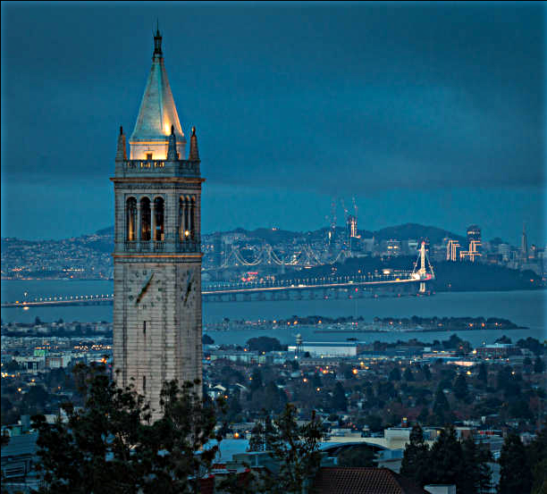
Using the same technique, I sharpened an image of the Berkeley night skyline, though I personally feel I still prefer the unsharpened version.

In this section of the project, we combine low and high frequencies to make hybrid images where the image changes depending on the distance you view it from.
To construct the hybrid images, we use techniques from the previous sections. More specifically, after aligning the images, we create a low frequency version of one image (the one viewed from afar) using a Gaussian filter. Then we create a high frequency version of the other image (the one viewed from up close) using the difference between the original image and the low passed image. Then, we average the two images, and get our final result.
The first hybrid image created was the one provided by the staff:
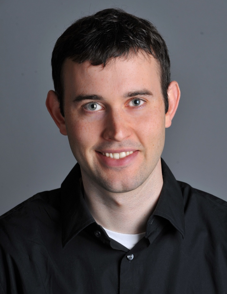
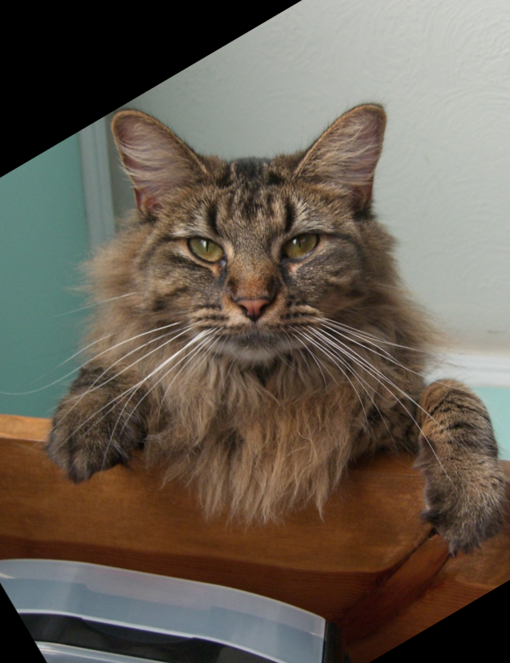
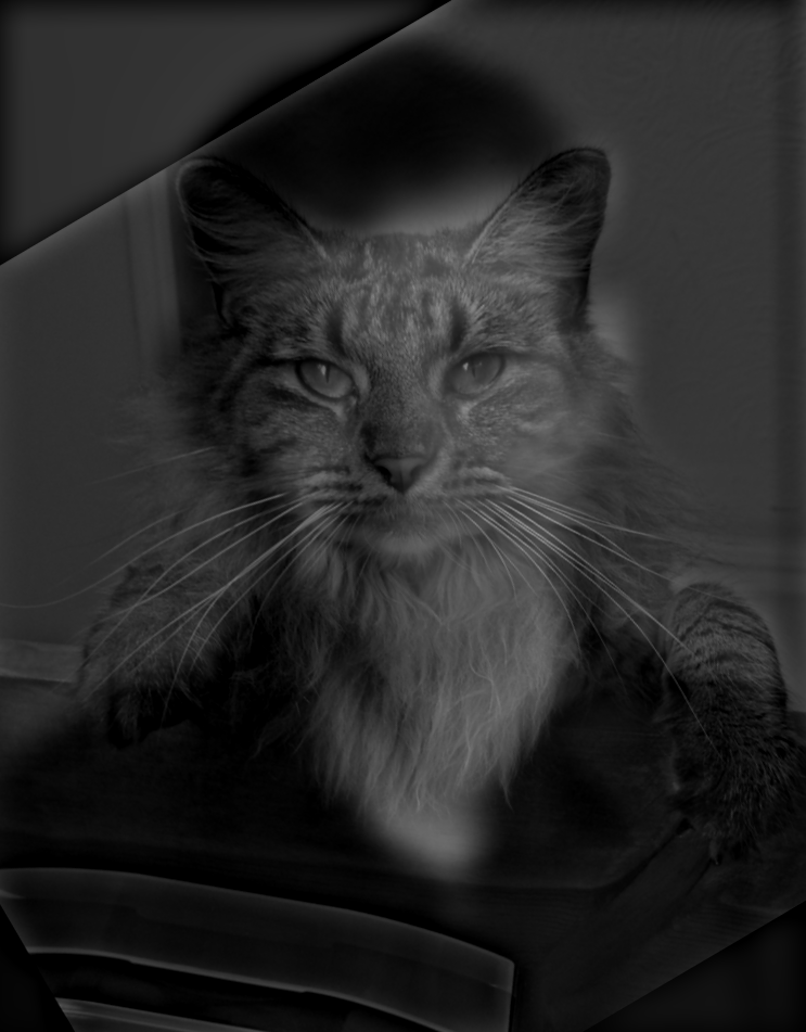
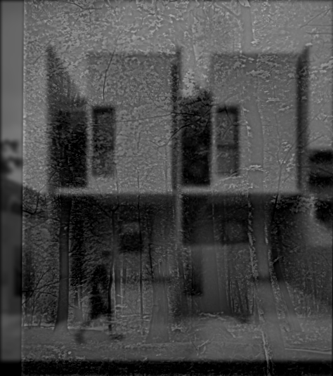
I also chose an intentionally mismatching set of images to show a potential difficult example: when the images don't structurally match up well and one image has many high frequencies:
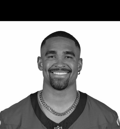
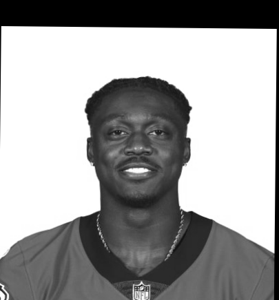
I think my best result was in mixing two football players on the Philadelphia Eagles: Jalen Hurts and AJ Brown. This proved more effective because I used headshots from each player, leading to matching angles, and since they are both humanoid, matching features as well. I think the most interesting thing is looking at their teeth, in my experience it looks like the hybrid image smiles wider when you get further (Hurts, the low pass, has a wider smile than Brown).
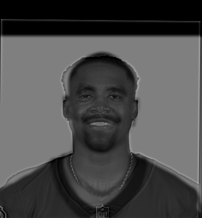
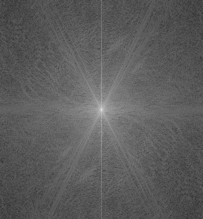
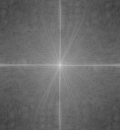
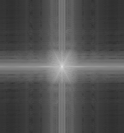
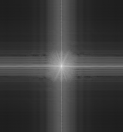
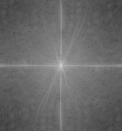
I also conducted my Fourier analysis on this hybrid image.
To set up our blending in the next section, in this section we create Gaussian and Laplacian stacks, which will us the blend different frequencies separately later on. To create the Gaussian stack, we simply apply a Gaussian filter successively to an image without downsampling. For demonstration, we apply it to both the apple and the orange:


The Gaussian stacks are then used to create the Laplacian stacks, which help divide the image into different frequencies. To create the Laplacian stack, we take the difference between each element in the Gaussian stack, and subtract it from the next most clear image in the stack. We also keep the bottom image of the Gaussian stack as the bottom of the Laplacian stack. Here are the min-max normalized Laplacian stacks:


Now that we have our Laplacian, we can blend some images. To do so, we create a mask; for the orange and apple, we use a mask with a simple vertical boundary. We then create a Gaussian stack with this mask (the displayed stack will have length 15, since that's what I decided on using for the oraple). For my Gaussian stack, I opted to actually create a length 16 stack, then throw out the original binary mask, because it was drawing a noticable line on my oraple.

Then, using the stack of masks, and the Laplacian stacks of both the orange and the apple, we use the following equation to blend:
$$LS_l(i, j) = GR_l(i, j) LA_l(i, j) + (1 - GR_l(i, j))LB_l(i, j)$$
Where $LS$ is the combined stack, $GR$ is the Gaussian stack of masks, $LA, LB$ are the Laplacian stacks, and $l$ is the layer. In essense, we multiply the first Laplacian stack by the Gaussian stack, the second Laplacian by 1 minus the Gaussian stack (at each element), and add them together to blend. This is done at each channel level individually.
Finally to make the blended image, we add up all layers of the stack for each image channel, then stack image channels to create our final image:
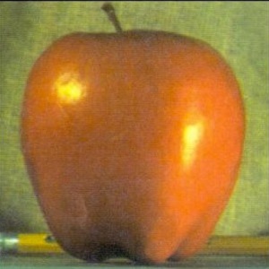
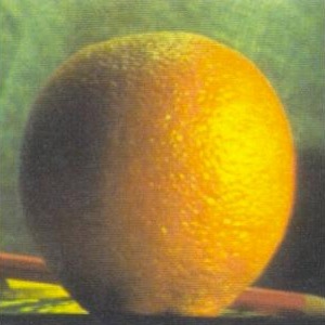
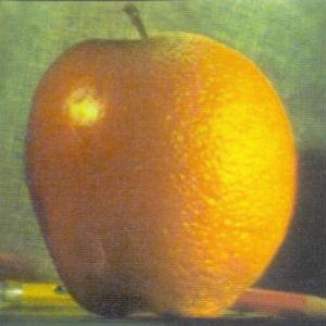
I made three additional blended images shown below.

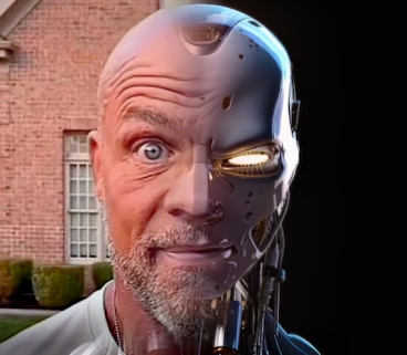
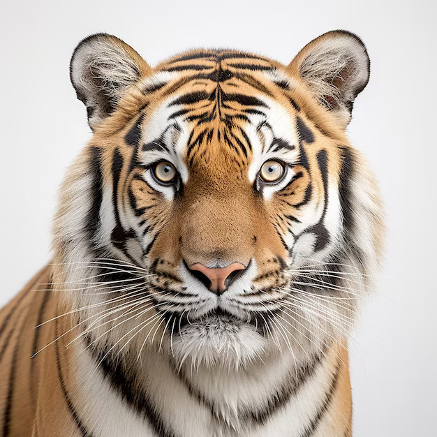
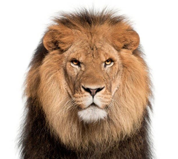
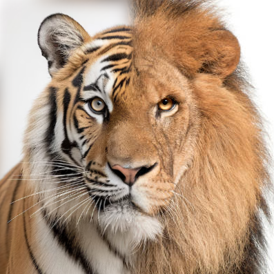
For the liger (my best result, probably because they line up structurally the best), we can see the final blended stack before being added up to better understand how we blend at multiple resolutions:

We can see that at higher frequencies on the right, there is minimal blend and more of a strict cutoff, while at the left side for the lower frequencies, the pictures tend to bleed into one another more. After adding this stack together and clipping values, we get the liger displayed above.