
Note: slideshows are not functional on .pdf version of this site and you won't be able to see all of my pictures.
In this project, we were asked to take scanned glass plate images from the Prokudin-Gorskii collection, and automatically overlay then using image processing techniques. In particular, we were given three color channels: R, G, and B, each of which were represented by a 2-dimensional matrix, and had to implement a procedure to evaluate what alignment of those channels would result in the most accurate final, single, RGB color image.
For the entire project, we align the three plates by taking the red and green plate and aligning them individually to the blue plate. After finding the displacements for those alignments, we take the displaced red and green plates and combine them both with the blue plate for our final image.
The simplest and most intuitive method of aligning the images is iterating over a displacement range and comparing all possible alignments across that range using some kind of similarity metric. For my naive approach, I chose to use mean squared error:
$$MSE(A, B) = \frac{1}{N} \sum_{i} \sum_{j} (A_{ij} - B_{ij})^2$$
The alignment function I wrote displaces images using the np.roll() function, which "rolls over" rows/columns when they leave the original
dimensions of the matrix, instead placing them in the same order at the opposite end of the matrix. It is important to note that the alignment scoring
does not make use of rolled over pixels in similarity scoring.
For smaller images, this can work very effectively by looking through a $[-15, 15]$ range of pixel displacements for both horizontal (shifting columns) and vertical (shifting rows) directions, since this range is not computationally prohibitive and still covers a large portion of the possible alignments.
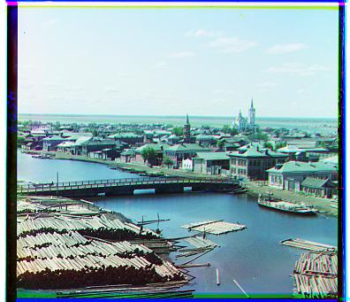
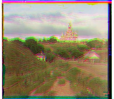
Through this naive method, we get decent results on tobolsk.jpg, but not on monastery.jpg and cathedral.jpg:


A possibility for why the last two pictures are misaligned even with $MSE$ scoring is that the borders of the raw plates are interfering with the accuracy of the scoring system. Combined with the fact that there also tends to be more distortion around the edges of the picture even past the borders, it seemed appropriate to crop the edges of the images before aligning so the alignment is focused on the focused center of the image. If the center is appropriately lined up, it follows that the remainder of the photo should be as well.
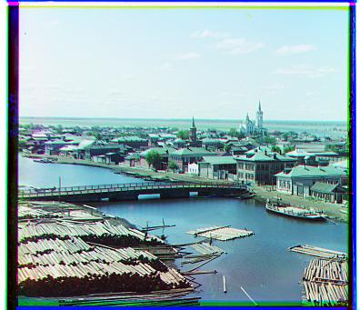
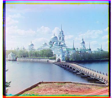
I specifically chose to take $7.5\%$ off of each side (left, right, top, bottom) of the images, then align. Then using the extracted displacements, I mapped the original, uncropped plates together. This netted significantly improved results on the smaller images.
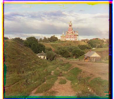
While the exhaustive search is effective for the smaller images because they are sized in the order of hundreds of pixels, it becomes ineffective for larger images in the order of thousands of pixels. This is because the $[15, 15]$ displacement range becomes inadequate in finding the best displacement, and increasing the range also drastically increases the runtime of the alignment function. Thus, a more efficient method of alignment is needed.
The solution was to implement a pyramid search, where we create an image pyramid by iteratively downsample the image several times, then work "down" the pyramid by finding displacements at lower resolutions, then carrying on the best displacement at that level to the next lowest level until we reach the original resolution. This makes the search process more efficient; we first find an approximately good displacement, move to a higher resolution, and starting from that approximate location, we can find an even better displacement, so on and so forth. While considering a large range of possible displacments we can still retain speed and accuracy.
The following are the results of my pyramid search:
Generally, a simple crop and $MSE$ alignment using a pyramid search is suitable for all the large images. The single exception is emir.tif, which has trouble aligning because the three color channels have very different color intensities on matching sections of the photograph. Thus, it may not be appropriate to use $MSE$ to match channels, since the blue and red channels specifically seem to have significant intensity differences.
The solution is to use a non-RGB based similarity metric, such as the structural similarity index measure (SSIM), which is instead based on the product luminance, constrast, and structure. The following explanation is paraphraphrased from Wikipedia.
Comparison of the luminance between images $x$ and $y$ uses the following formula:
$$l(x, y) = \frac{2\mu_x \mu_y + c_1}{\mu_x^2 + \mu_y^2 + c_1}$$
Where $\mu_x$ and $\mu_y$ are the pixel sample means of $x$ and $y$ and $c_1$ is a constant used to stabilize the division. When $\mu_x = \mu_y$, the comparison formula results in $1$, and the further apart the sample means are, the smaller $l(x, y)$ is.
Similarly, comparison of the contrast between images $x$ and $y$ uses the following formula:
$$c(x, y) = \frac{2\sigma_x \sigma_y + c_2}{\sigma_x^2 + \sigma_y^2 + c_2}$$
Where $\sigma_x$ and $\sigma_y$ are the sample variances of $x$ and $y$ and $c_2$ is a different constant used to stabilize the division. In the same way as luminance, when $\sigma_x = \sigma_y$, the comparison formula results in $1$, and the further apart the sample means are, the smaller $c(x, y)$ is.
Finally, comparison of the structure between images $x$ and $y$ uses the following formula:
$$s(x, y) = \frac{\sigma_{xy} + c_3}{\sigma_x^2\sigma_y^2 + c_3}$$
Where $\sigma_{xy}$ is the covariance of $x$ and $y$ and $c_3$ is a different constant used to stabilize the division ($c_3 = c_2/2$). This similarity score is 1 when $x$ and $y$ are perfectly correlated, and the less correlated they are the lower the score. Without the constants, this similarity score is the definition of the correlation between $x$ and $y$.
Thus, $SSIM$ measures the similarity between two planes based on factors other than direct intensity, which we hope will give better results on an edge
case like emir.tif. I implemented $SSIM$ by using sk.metrics.structural_similarity() (sadly no bells and whistles here).
A large disadvantage of $SSIM$ as a metric is that it takes much longer to run than $MSE$, even when optimized. While $MSE$ based pyramid search generally took less than 30 seconds per photo, $SSIM$ based pyramid search typically took around 5 minutes on larger images. Thus, I only ran $SSIM$ on a few images.
The following are the results of my pyramid search using $SSIM$:
While emir.tif drastically improved, most other images I tested saw no improvement, with only one pixel differences in the two alignments. The exception was three_generations.tif, which had a larger difference between $SSIM$ and $MSE$, but contrary to emir.tif, seemed better using $MSE$, if only marginally (and unscientifically based on my and my housemates' opinions). Below is a side-by-side for easier comparison if you would like to stare at it and find the very small differences:
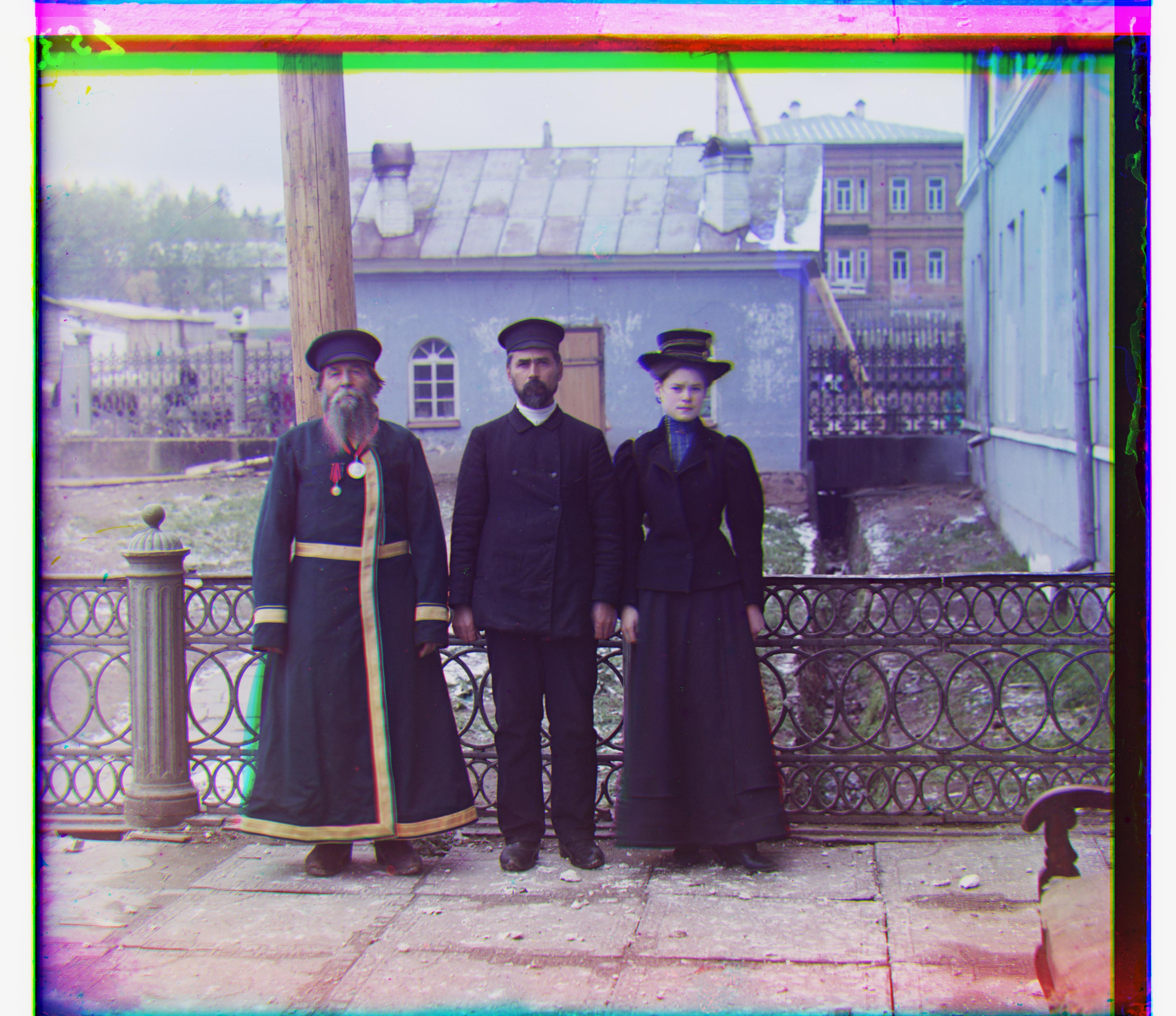

The final step I took during this project was to post-process the images to attempt to clean off the abnormally colored edges through doing two things. First, I implemented a more dynamic cropping function using canny edge detectors to try and find the borders. Second, I automatically cropped all rolled over pixels.
To implement the Canny edge detector, I used the skimage.feature.canny() function with $\sigma=5$ to avoid reading too much noise during
edge detection. I also created a mask so that we only detect edges in the extremeties of the image. I chose to use a mask that that takes $7.5\%$ off of
each side, similar to my naive constant crop, with the idea being in the worst case the Canny filter based prop would only crop as much as the naive crop.
Since this is a post-processing crop, I'm more ambivalent to accidentally including some borders and distorted areas, I prioritize capturing as much
of the image as possible while still removing noticable borders.
After retrieving the edges, I go to each border of the image (the respective $7.5\%$ areas), and take the median index along the axis perpendicular to the side we are cropping (ex. for cropping the top, we retrieve the mean index for edges along the vertical axis). This median index is where I choose to crop.
The mains struggle ended up being cases where the white border was cropped, but the black border remained. This was fairly common and a current limitation of my heuristic approach to identifying what index to cut.
Below are some comparisons of the original image (on the left), the Canny based crops (in middle) and the naive, constant crops (on the right) on the blue channels on some images.
The last step was to remove the roll over pixels from the final image (which significantly improved the border issues). The final images and their shifts are below (all using $MSE$ except for emir.tif, which uses $SSIM$).